Owl is an OCaml numerical library. It supports both dense and sparse matrix operations, linear algebra, regressions, and many advanced mathematical and statistical functions (such as Markov chain Monte Carlo methods).
The full documentation is here: Owl Manual
If you have any questions, please email to liang.wang@cl.cam.ac.uk
or message me on: Twitter, Google+, Facebook, Blogger, LinkedIn
Installation is rather trivial. First, you need to clone the repository.
git clone git@github.com:ryanrhymes/owl.gitThen you need to install all the dependencies. Owl depends on gsl, ctypes, plplot, and several other modules. Check the _oasis file in the owl folder to find out the complete list of required modules.
Next, you can compile and install the module with the following command.
make oasis
make && make install
Owl is well integrated with utop. Now you can start utop and continue this tutorial to do some experiments. If you want utop to automatically load Owl for you, you can also edit .ocamlinit file in your home folder by adding the following lines.
#require "Owl"If you are too lazy to do any labour work, here is a docker image to let you try Owl without dealing with aforementioned installation and configuration steps. The docker image is automatically build from the master branch whenever there are new commits. You can check the building history on Docker Hub.
Just pull the image, start a container, then play with it in utop. The latest source code is saved in /root/owl directory.
docker pull ryanrhymes/owl
docker run -t -i ryanrhymes/owlOwl currently has seven core modules and their names all start with Owl_ to avoid name conflicts, e.g., Owl_dense, Owl_sparse, Owl_maths, Owl_stats, and etc. After utop successfully loads Owl library, you can access the module functions using aforementioned names.
However, a more convenient way is to use Owl module as an entry point which provides aliases of the core module names for easy access, e.g., Owl.Dense is the same as Owl_dense, and Owl.Regression is the same as Owl_regression. Given no name conflicts, you can simply open the whole Owl module for convenience as I will do in the rest of this tutorial.
Dense module supports dense matrix operations while Sparse module supports sparse ones. To start, we can use Dense.uniform_int to create a 5x5 random dense matrix.
let x = Dense.uniform_int 5 5;;You should see the following output in utop.
   C0 C1 C2 C3 C4
R0 25  2 77 85 72
R1 71 92 98 87 53
R2 35 29 82 65 20
R3  2 29 66 42 12
R4 99 72 78 30 11
val x : Dense.dsmat =
Dense module also provides other functions to create various matrices, e.g., as below.
let x = Dense.eye 5;;             (* identity matrix *)
let x = Dense.zeros 5 5;;         (* all elements are zeros *)
let x = Dense.ones 5 5;;          (* all elements are ones *)
let x = Dense.uniform 5 5;;       (* random matrix of uniform distribution *)
let x = Dense.gaussian 5 5;;      (* random matrix of gaussian distribution *)
...
Combined with Stats module, you can also create any matrices of many distributions. E.g., the following code first creates an empty dense matrix, then initialise the elements with Bernoulli distribution. Test it in utop, you should get a dense matrix where half of the elements are zeros.
let x = Dense.empty 8 8 |> Dense.map (fun _ -> Stats.Rnd.bernoulli 0.5 |> float_of_int);;Or create a matrix where the elements follow Laplace distribution.
let x = Dense.empty 8 8 |> Dense.map (fun _ -> Stats.Rnd.laplace 0.2);;With Dense module, you can also generate linearly spaced interval and meshgrids, e.g.,
let x = Dense.linspace 0. 5. 6;;which will return a 1x5 row vector as below
   C0  C1  C2  C3  C4  C5
R0  0   1   2   3   4   5
val x : Dense.dsmat =
Matrices can be saved to and loaded from a file.
Dense.save x 'matrix_01.data';;  (* save the matrix to a file *)
Dense.load 'matrix_01.data';; (* load the matrix from a file *)Both Dense and Sparse modules provide a wide range of operations to access the elements, rows, and columns of a matrix. You can use Dense.set and Dense.get to manipulate individual element.
Dense.set x 0 1 2.5;;
Dense.get x 0 1;;
Equivalently, there are shorthands for Dense.get and Dense.set.
x.{0,1} <- 2.5;;  (* Dense.set x 0 1 2.5 *)
x.{0,1};;         (* Dense.get x 0 1 *)
We can use Dense.row and Dense.col to retrieve a specific row or column of a matrix, or use Dense.rows and Dense.cols to retrieve multiple of them.
Dense.row x 5;;        (* retrieve the fifth row *)
Dense.cols x [|1;3;2|] (* retrieve the column 1, 3, and 2 *)
E.g., the following code generates a random matrix, then scales up each element by a factor of 10 using Dense.map function.
let x = Dense.(uniform 6 6 |> map (fun x -> x *. 10.));;We can iterate a matrix row by row, or column by column. The following code calculates the sum of each row by calling Dense.map_rows function.
let x = Dense.(uniform 6 6 |> map_rows sum);;We can fold elements by calling Dense.fold, fold rows by calling Dense.fold_rows. Similarly, there are also functions for filter operations. The following code filters out the elements not greater than 0.1 in x.
Dense.filter ((>) 0.1) x;; (* not greater than 0.1 in x *)We can also do something more complicated, e.g., by filtering out the rows whose summation is greater than 3.
Dense.filter_rows (fun r -> Dense.sum r > 3.) x;;Shuffle the rows and columns, or draw some of them from a matrix.
Dense.shuffle_rows x;;                (* shuffle the rows in x *)
Dense.draw_cols x 3;;                 (* draw 3 columns from x with replacement *)
...
Practically, Sparse module provides all the similar operations for sparse matrices. In addition, Sparse module also has extra functions such as only iterating non-zero elements Sparse.iter_nz, and etc. Please read the full documentation for details.
Simple matrix mathematics like add, sub, multiplication, and division are included in Dense module. Moreover, there are predefined shorthands for such operations. E.g., the following code creates two random matrices then compare which is greater.
let x = Dense.uniform 6 6;;
let y = Dense.uniform 6 6;;
Dense.(x >@ y)                  (* is x greater than y? *)
Dense.(x =@ y)                  (* is x equal to y? *)
...
Some basic math operations includes:
Dense.(x +@ y)                  (* add two matrices *)
Dense.(x *@ y)                  (* multiply two matrices, element-wise *)
Dense.(x $@ y)                  (* dot product of two matrices *)
Dense.(x +$ 2.)                 (* add a scalar to all elements in x *)
...
Apply various functions in Maths module to every element in x
Dense.(Maths.sin @@ x);;        (* apply sine function *)
Dense.(Maths.exp @@ x);;        (* apply exponential function *)
...
Concatenate two matrices, vertically or horizontally by
Dense.(x @= y);;                (* equivalent to Dense.concat_vertical *)
Dense.(x @|| y);;               (* equivalent to Dense.concat_horizontal *)
More advanced linear algebra operations such as svd, qr, and cholesky decomposition are included in Linalg module.
let u,s,v = Linalg.svd x   (* singular value decomposition *)
let q,r = Linalg.qr x      (* QR decomposition *)
let l = Linalg.cholesky x  (* cholesky decomposition *)
...
Regression module currently includes linear, exponential, nonlinear, ols, ridge, lasso, svm, and etc. Most of them are based on a stochastic gradient descent algorithm implemented in Optimise module.
In the following, let's use an example to illustrate the simplest linear regression in Regression module. First, let's generate the measurement x which is a 1000 x 3 matrix. Each row of x is an independent measurement.
let x = Dense.uniform 1000 3;;Next let's define the parameter of a linear model, namely p, a 3 x 1 matrix.
let p = Dense.of_array [|0.2;0.4;0.8|] 3 1;;Then we generate the observations y from x and p by
let y = Dense.(x $@ p);;Now, assume we only know x and y, how can we fit x and y into a linear model? It is very simple.
let p' = Regression.linear x y;;From utop, you can see that p' equals [|0.2; 0.4; 0.8|] which is exactly the same as p. For other regression such as lasso and svm, the operation is more or less the same, please read Owl document for details.
There is another separate Tutorial on Plotting in Owl.
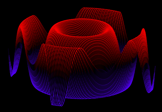
Herein, let's use an example to briefly show how to plot the result using Plot module. We first generate two mesh grids then apply sine function to them by using the operations introduced before.
let x, y = Dense.meshgrid (-2.5) 2.5 (-2.5) 2.5 100 100 in
let z = Dense.(Maths.sin @@ ((x **@ 2.) +@ (y **@ 2.))) in
Plot.mesh x y z;;
No matter what plot terminal you use, you should end up with a figure as below.
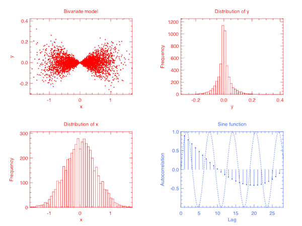
Besides Plot.mesh, there are several other basic plotting functions in Plot. Even though the module is still immature and under active development, it can already do some fairly complicated plots with minimal coding efforts. E.g., the following code will generate a 2 x 2 subplot.
let f p i = match i with
  | 0 -> Stats.Rnd.gaussian ~sigma:0.5 () +. p.(1)
  | _ -> Stats.Rnd.gaussian ~sigma:0.1 () *. p.(0)
in
let y = Stats.gibbs_sampling f [|0.1;0.1|] 5_000 |> Dense.of_arrays in
let h = Plot.create ~m:2 ~n:2 "test_plot_04.png" in
let _ = Plot.set_background_color h 255 255 255 in
let _ = Plot.subplot h 0 0 in
let _ = Plot.set_title h "Bivariate model" in
let _ = Plot.scatter ~h (Dense.col y 0) (Dense.col y 1) in
let _ = Plot.subplot h 0 1 in
let _ = Plot.set_title h "Distribution of y" in
let _ = Plot.set_xlabel h "y" in
let _ = Plot.set_ylabel h "Frequency" in
let _ = Plot.histogram ~h ~bin:50 (Dense.col y 1) in
let _ = Plot.subplot h 1 0 in
let _ = Plot.set_title h "Distribution of x" in
let _ = Plot.set_ylabel h "Frequency" in
let _ = Plot.histogram ~h ~bin:50 (Dense.col y 0) in
let _ = Plot.subplot h 1 1 in
let _ = Plot.set_foreground_color h 51  102 255 in
let _ = Plot.set_title h "Sine function" in
let _ = Plot.plot_fun ~h ~line_style:2 Maths.sin 0. 28. in
let _ = Plot.autocorr ~h (Dense.sequential 1 28) in
Plot.output h;;
The end result is as follows. You probably have already grasped the idea of how to plot in Owl. But I promise to write another separate post to introduce plotting in more details.
There are a lot of basic and advanced mathematical and statistical functions in Maths and Stats modules. Most of them are interfaced to Gsl directly, so you may want to read GSL Manual carefully before using the module.
Stats has three submodules: Stats.Rnd for random numbers, Stats.Pdf for probability dense functions, and Stats.Cdf for cumulative distribution functions. In addition, I have implemented extra functions such as two ranking correlations: Stats.kendall_tau and Stats.spearman_rho); two MCMC (Markov Chain Monte Carlo) functions in Stats module: Metropolis-Hastings (Stats.metropolis_hastings) and Gibbs sampling (Stats.gibbs_sampling) algorithms.
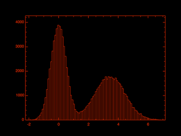
E.g., the following code first defines a probability density function f for a mixture Gaussian model. Then we use Stats.metropolis_hastings to draw 100_000 samples based on the given pdf f, and the initial point is 0.1. In the end, we call Plot.histogram to plot the distribution of the samples, from which we can clearly see they are from a mixture Gaussian model.
let f p = Stats.Pdf.((gaussian p.(0) 0.5) +. (gaussian (p.(0) -. 3.5) 1.)) in
let y = Stats.metropolis_hastings f [|0.1|] 100_000 |>  Dense.of_arrays in
Plot.histogram ~bin:100 y;;
The histogram below shows the distribution of the samples.
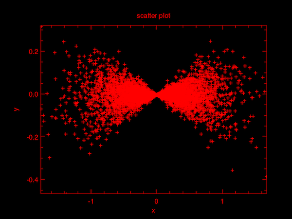
Here is another example using Stats.gibbs_sampling to sample a bivariate distribution. Gibbs sampling requires the full conditional probability function so we defined its corresponding random number generator in f p i where p is the parameter vector and i indicates which parameter to sample.
let f p i = match i with
  | 0 -> Stats.Rnd.gaussian ~sigma:0.5 () +. p.(1)
  | _ -> Stats.Rnd.gaussian ~sigma:0.1 () *. p.(0)
in
let y = Stats.gibbs_sampling f [|0.1;0.1|] 5_000 |> Dense.of_arrays in
Plot.scatter (Dense.col y 0) (Dense.col y 1);;
We take 5000 samples from the defined distribution and plot them as a scatter plot, as below.
The future plan is to embed a small PPL (Probabilistic Programming Language) in Stats module.
Owl is under active development, and I really look forward to your comments and contributions. Besides setting up a complete development environment on your native system, the easiest way to contribute is to use the Owl Docker Image. Just pull the image and dig into code saved in /root/owl, then have fun!


