This is the Spring 2017, Harvard Statistics 149: Generalized Linear Models prediction contest/course project.
The goal of this project is to use the modeling methods in Statistics 149 (and possibly other related methods) to analyze a data set on whether a Colorado voting-eligible citizen ended up actually voting in the 2016 US election. These data were kindly provided by moveon.org. The competition can be found here and ended April 30, 2017, at 10pm EDT.
Based on our analysis of the data, individuals who fall into the following categories are more likely to vote:
- Individuals that are more likely to be married are more likely to vote
- A very low and a very high likelihood of having children are more likely to vote
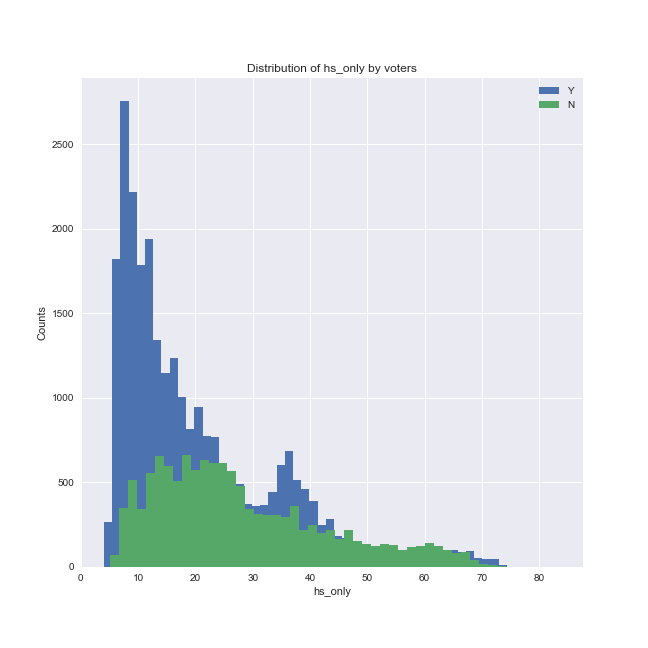
- Those who are more likely to vote have a low likelihood of only having a high school degree
Individuals in the following categories are less likely to vote and could therefore be targeted for voter turnout campaigns:
- As the number of days since registration increases, an individual becomes less likely to vote
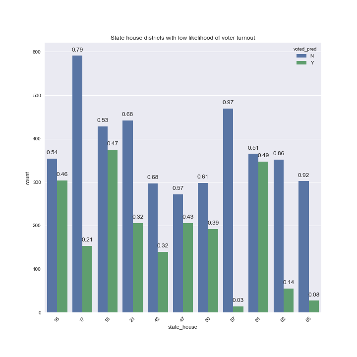
- Citizens in certain state house districts are less likely to vote relative to other districts
Below we list the predictor variables and our findings regarding each from the initial exploration of the data:
- voted: This is the (binary) response variable and denotes whether an individual did (Y) or did not (N) vote. ~67.8% of individuals did vote (80,357) compared to ~32.2% who did not vote (38,172). This class imbalance is important to keep in mind for model fitting, as certain models do not handle imbalanced classes well.
- gender: Gender is coded as a 3 level factor (female, male, unknown). Females (58,414) and males (59,916) are equally represented in the dataset, and only 199 are unknown.
- congress_district: Congressional district the voter is registered in; this is a 7 level factor with 2 missing values. These missing values are not a concern as they represent an insignificant portion of the data.
- state_house: State house district the voter is registered in; a 65 level factor with 2 missing values. The large number of levels may make incorporation of this predictor difficult if using a dummy coding schema.
- age: Age in years of the voter; no missing or bizarre values
- dist_ballot: Distance from closest ballot drop-off location in miles. 113,247 values are missing, or ~95.5% of the data. This is significant and was addressed via imputation in this notebook. Note that in the final model imputation actually led to worse performance than simply dropping these variables, likely due to the large percentage of data that needed to be imputed.
- dist_poll: Distance in miles to voter's polling place; same missing values as dist_ballot
- party: D=Democrat, R=Republican, L=Libertarian, G=Green, O=American Constitutional Party, U=Unaffiliated
- race: 11 level factor, including Uncoded.
- hs_only: Score for likelihood of having high school as highest completed degree
- married: Score for likelihood of being married
- children: Score for likelihood of having children at home
- cath: Score for likelihood of being Catholic
- evang: Score for likelihood of being Evangelical
- non_chrst: Score for likelihood of being non-Christian
- other_chrst: Score for likelihood of being another form of Christian
- likelihood scores were all caculated from proprietary models
- days_reg: Number of days since the individual registered as a voter; no missing or bizarre values
Below are the summary statistics for our quantitative variables grouped by whether the citizen voted (Y) or did not vote (N):
| voted_Y | age | dist_ballot | dist_poll | hs_only | married | children | cath | evang | non_chrst | other_chrst | days_reg |
|---|---|---|---|---|---|---|---|---|---|---|---|
| count | 80357.0 | 3897.0 | 3897.0 | 80357.0 | 80357.0 | 80357.0 | 80357.0 | 80357.0 | 80357.0 | 80357.0 | 80357.0 |
| mean | 37.0 | 3.0 | 3.0 | 22.0 | 48.0 | 34.0 | 12.0 | 16.0 | 40.0 | 31.0 | 453.0 |
| std | 16.0 | 2.0 | 2.0 | 15.0 | 33.0 | 22.0 | 6.0 | 7.0 | 11.0 | 4.0 | 108.0 |
| min | 18.0 | 2.0 | 2.0 | 4.0 | 3.0 | 1.0 | 5.0 | 2.0 | 5.0 | 9.0 | 223.0 |
| 25% | 24.0 | 2.0 | 2.0 | 10.0 | 16.0 | 16.0 | 9.0 | 10.0 | 32.0 | 29.0 | 371.0 |
| 50% | 32.0 | 2.0 | 2.0 | 17.0 | 46.0 | 28.0 | 12.0 | 15.0 | 39.0 | 31.0 | 441.0 |
| 75% | 47.0 | 3.0 | 3.0 | 30.0 | 76.0 | 49.0 | 15.0 | 21.0 | 48.0 | 34.0 | 536.0 |
| max | 101.0 | 29.0 | 29.0 | 84.0 | 100.0 | 90.0 | 74.0 | 56.0 | 74.0 | 51.0 | 677.0 |
| voted_N | age | dist_ballot | dist_poll | hs_only | married | children | cath | evang | non_chrst | other_chrst | days_reg |
|---|---|---|---|---|---|---|---|---|---|---|---|
| count | 38172.0 | 1385.0 | 1385.0 | 38172.0 | 38172.0 | 38172.0 | 38172.0 | 38172.0 | 38172.0 | 38172.0 | 38172.0 |
| mean | 33.0 | 3.0 | 3.0 | 25.0 | 36.0 | 32.0 | 12.0 | 16.0 | 41.0 | 31.0 | 472.0 |
| std | 14.0 | 2.0 | 3.0 | 15.0 | 28.0 | 18.0 | 7.0 | 6.0 | 10.0 | 4.0 | 111.0 |
| min | 18.0 | 2.0 | 2.0 | 4.0 | 3.0 | 1.0 | 5.0 | 2.0 | 5.0 | 10.0 | 223.0 |
| 25% | 22.0 | 2.0 | 2.0 | 13.0 | 13.0 | 18.0 | 8.0 | 11.0 | 34.0 | 29.0 | 383.0 |
| 50% | 28.0 | 2.0 | 2.0 | 22.0 | 24.0 | 27.0 | 11.0 | 15.0 | 41.0 | 31.0 | 466.0 |
| 75% | 39.0 | 3.0 | 3.0 | 35.0 | 59.0 | 44.0 | 14.0 | 20.0 | 48.0 | 33.0 | 567.0 |
| max | 99.0 | 46.0 | 46.0 | 84.0 | 100.0 | 89.0 | 73.0 | 50.0 | 73.0 | 47.0 | 677.0 |
On average, people who voted may be slightly older and have a higher likelihood of being married than those who did not vote (although the standard deviations are large). As mean values can be skewed by extreme values, below we also display the median values:
| voted | age | dist_ballot | dist_poll | hs_only | married | children | cath | evang | non_chrst | other_chrst | days_reg |
|---|---|---|---|---|---|---|---|---|---|---|---|
| N | 28 | 2.26 | 2.42 | 21.7 | 23.7 | 27.4 | 11.0 | 15.3 | 40.8 | 31.0 | 466 |
| Y | 32 | 2.28 | 2.45 | 17.3 | 46.0 | 27.5 | 12.0 | 15.0 | 39.2 | 31.4 | 441 |
Age and hs_only also differ the most in terms of the median, further suggesting these may be important predictors. Next we can look at the correlations between our variables:
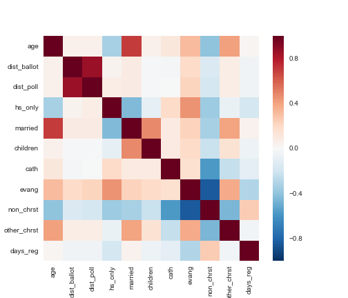
The correlation matrix shows expected correlations, e.g., dist_poll and dist_ballot are highly correlated, as are age and likelihood of being married, while likelihood of being non-Christian is anti-correlated with likelihood of being some form of Christian. Most other pair-wise correlations appear relatively weak.
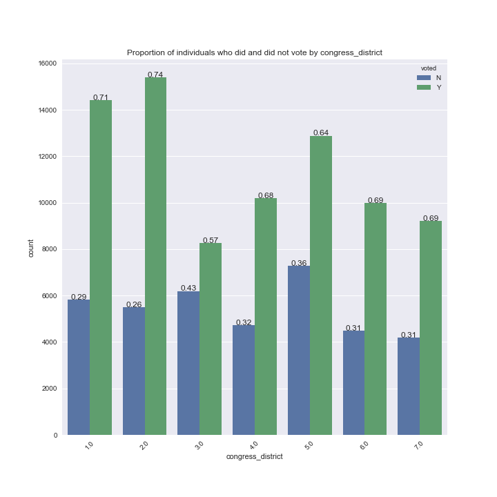
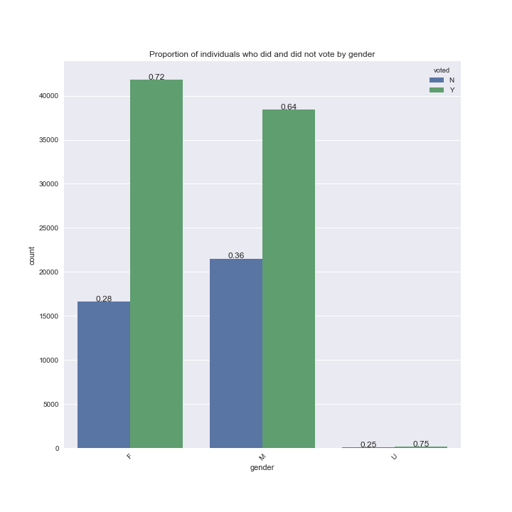
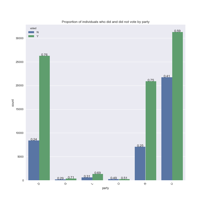
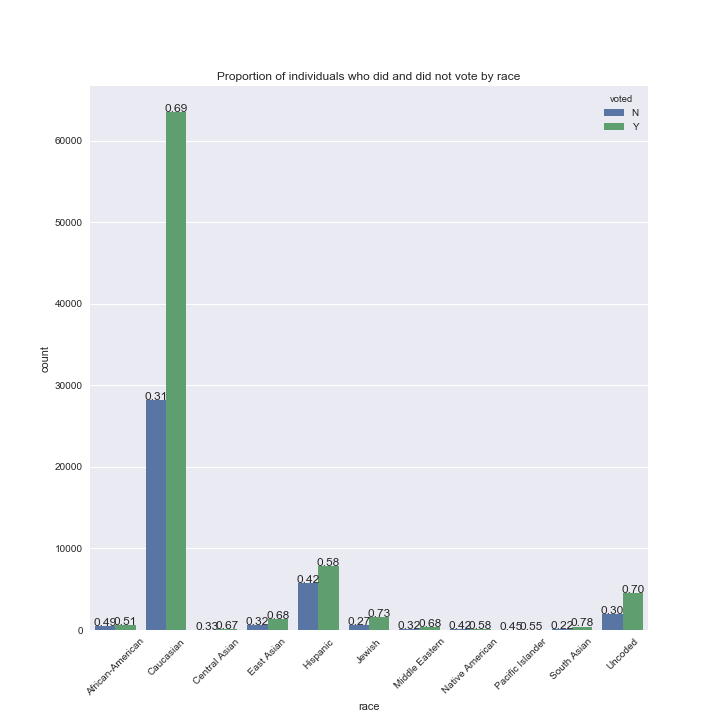
To investigate the relationship between the likelihood of voting and our categorical variables (congressional district, gender, party, race and state house district), we can plot the proportion of individuals in each category who did and did not vote.
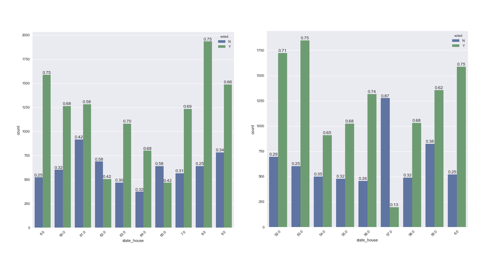
The ratio of those who did and did not vote in each category of our categorical variables are generally between 3:1 and 2:1. For example, ~72% of women and ~64% of men voted in Colorado in 2016, thus the likelihood of an individual voting given their gender alone is similar. There are too many state house districts to plot each individually, but there are some state house districts where the proportion of citizens who did and did not vote differed (see below):
In the next notebook we explored features that could potentially be useful for predicting voter turnout by training a naive random forest classifier with observations containing no missing values and examining which features the classifier used to split the data.
| features | importance |
|---|---|
| dist_ballot | 0.0756 |
| children | 0.07282 |
| state_house | 0.06987 |
| congress_district | 0.06753 |
| dist_poll | 0.06684 |
| age | 0.06652 |
| race | 0.06569 |
| party | 0.06559 |
| married | 0.0649 |
| hs_only | 0.06433 |
| gender | 0.05802 |
| cath | 0.0132 |
| other_chrst | 0.00662 |
| days_reg | 0.0066 |
| non_chrst | 0.00574 |
| evang | 1e-05 |
Based on these results, it seemed distance from ballot drop off location and polling place had good predictive power, and we therefore attempted multiple imputation by chained equations (MICE) here, though as already noted in our final model simply removing these variables resulted in better predictions than the imputed data. Removing the least important features in the table above did not result in an improved cross-validation log-loss score by the naive random forest.
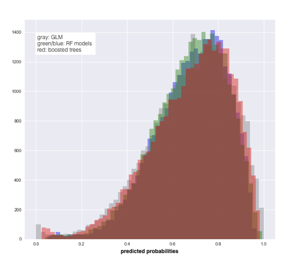
To predict voter turnout, we next fit a variety of classifiers in this notebook. Our initial models were logistic regression with L2 regularization and random forests with different tuned hyperparameters, followed by gradient boosted trees, which led to the largest drop in log-loss. To get a sense of what kind of predictions each fitted model was making, we can plot the distribution of the predicted probabilities of the different random forests, logistic regression and boosted tree models.
Although the predictions of all four models are similar overall, there are probability ranges where the models perform differently. For example, logistic regression makes the most extreme predictions, likely contributing to its poor performance. To overcome the weaknesses of any individual model, ensemble models, where the final prediction is a weighted average or vote of each classifier, and stacking, which takes the probability predictions from individually tuned models and using these probabilities as a training set for a meta-classifier to produce final predictions, can be tested. Of the two methods, stacking led to the best final predictions on this dataset. I finished 5th out of 40 teams (100 students total).
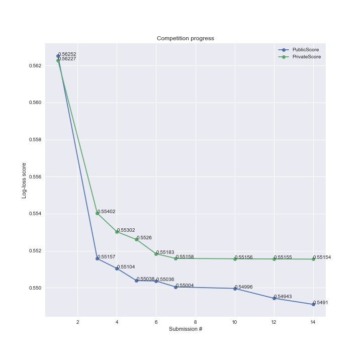
We can see competition progress on both the public and private leaderboards below:
The largest drop in log-loss was when we moved from a random forest to a gradient boosted tree model implemented via gradient boosted tree (submission 1 vs. submission 3). Further tuning of the gradient boosted tree model led to a significant decrease in both private and public log-loss scores (submissions 4-6). In submissions 7 and 10 we tested ensemble and stacked models, which led to modest improvements relative to gradient boosted tree alone. In the final two submissions, the decrease in log-loss was greater for the public score than the private score, suggesting that overfitting to the public leaderboard data may have started to occur.
- With such a large proportion of missing data in the dist_ballot and dist_poll variables, it would have been better to simply remove them from the dataset than to attempt imputation
- Imputation may have been better for the uncoded/unknown categories in race and gender, as a much smaller proportion of these variables were missing
- Fitting a generalized additive model (GAM) would have been a superior approach compared to logistic regression, as the former could have captured complex non-linear relationships in the voter data
- Cross-validation should ideally be performed with different random seeds to prevent overfitting
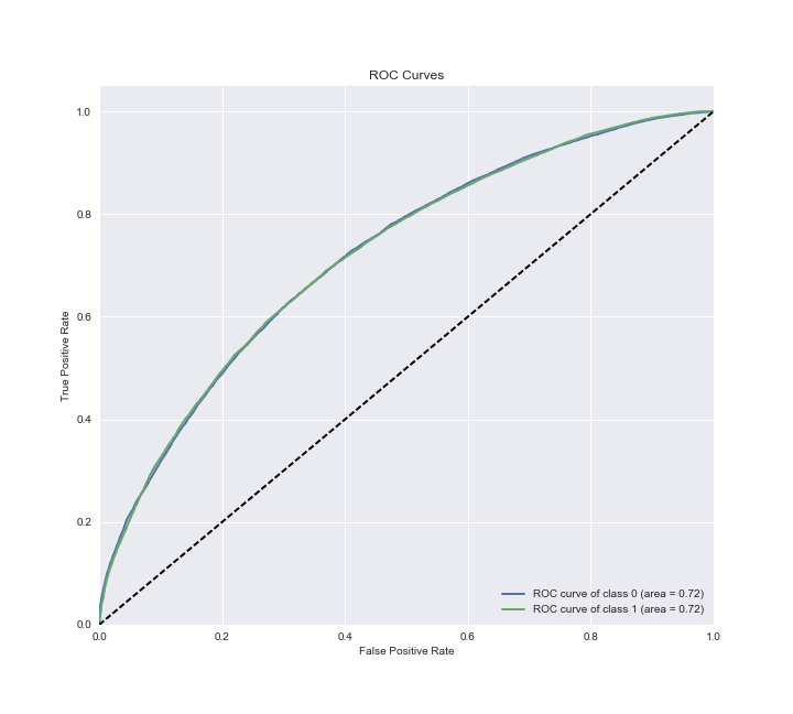
Ultimately the goal of this project is to predict, and potentially understand, whether a Colorado voter participated in the 2016 election (see this notebook). An important first step in achieving this goal is to decide on a probability threshold above which an observation will be scored as a positive case (will vote) and below which will be scored as a negative case (will not vote). Generally, domain knowledge and constraints need to be employed to determine the ideal threshold. For example, if the goal is to encourage as many voters as possible to participate in an election, then setting a higher threshold so that more people are classified as unlikely to vote may be appropriate, as these people can then be targeted for get-out-the-vote campaigns. On the other hand, in the real world there are always budget constraints, and therefore setting a lower threshold to target the individuals most ‘at risk’ of not voting may be a better use of limited resources. Plotting the true positive rate (TPR) vs. the false positive rate (FPR) on the test set to generate an ROC curve can help determine a threshold to optimize a given objective.
We will assume the test set contained a similar proportion of individuals who did and did not vote as the training set and selected a cutoff value that led to a ratio of positive and negative cases of approximately 2:1. This threshold is 0.61 and leads to classification of 26,932 observations in the test set as people who are likely to vote and 12,578 as those who are unlikely to vote. Using this threshold gives a TPR of about 0.77 and a FPR of about 0.47.
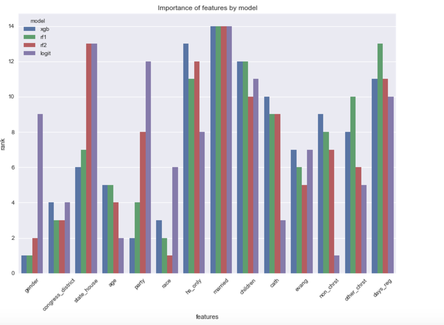
Ranking the importance scores from our tree-based models and coefficient magnitudes from the logistic regression results in the following plot:
All four models predict the likelihood of being married as the most important variable for classification. From the logistic regression, we can interpret the coefficient as a 0.1 increase in the likelihood score of being married results in an increased probability of ~0.61 of voting on the logit scale, all other predictors being equal. Although the actual magnitude of effect of married is different in the final stacked classifier, we can get a sense that the likelihood of being married has a strong effect on the likelihood of voting.
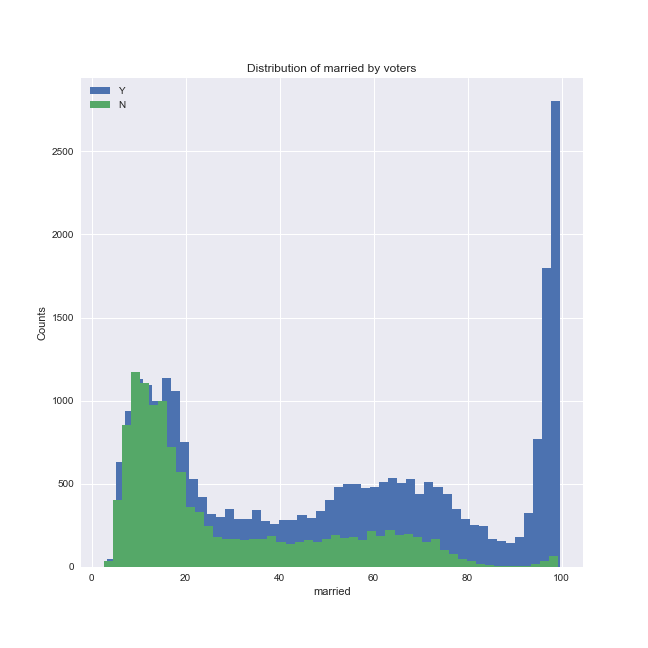
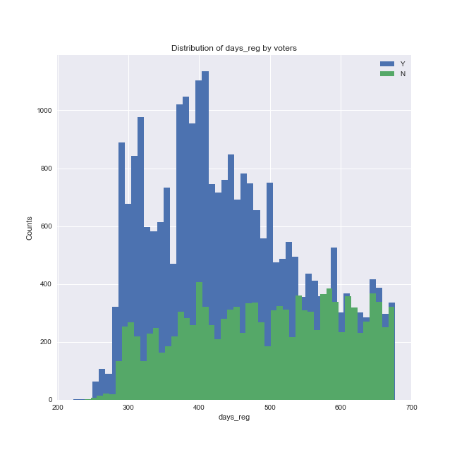
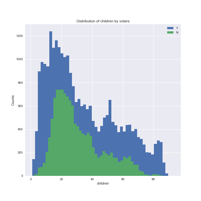
There is less 'consensus' amongst the four models as to the other predictors, although hs_only, children and days_reg generally ranked high. Let's plot married and these three variables grouped by whether the model predicted the individual is likely to vote or not.
We can see that there is a shift in the distribution of these predictors depending on whether the individuals were predicted to vote or not (note that in the plots above, the 'Y' group is plotted in blue and the 'N' group is plotted in green, in contrast to the other plots). The final stacked model predicts that:
- individuals with higher marriage likelihood scores are more likely to vote than not vote
- as the number of days since registration increases, the proportion of those who are unlikely to vote increases
- a very low and a very high likelihood score of having children are associated with an increased likelihood of voting
- those who are likely to vote are overrepresented in the low hs_only score range; in other words, a low likelihood of only having a high school degree corresponds to a high likelihood of voting
In addition to the features described above, state_house was ranked as the second most important feature from one of the random forest classifiers and also had a large coefficient magnitude in logistic regression. Investigating this feature we can see that certain state house districts are predicted to have relatively low voter turnout.
There are 11 state house districts where voter turnout is predicted to be very low, particularly in districts 57, 65 and 62.
In summary, the final model predicts that a Colorado voter with a low likelihood of being married, a longer period since voter registration, a moderately low likelihood of having children, a higher likelihood score of only have a high school degree and who lived in certain state house districts were the least likely to vote in the 2016 election. Individuals that fall within one or several of these categories could be targeted for voter turnout campaigns in future elections. Importantly, analysis of variables in this notebook was based off a particular threshold, and these could change depending on the threshold for predicting whether an individual will or will not vote. Another caveat to keep in mind is that there is an assumption that voter turnout and the variables driving it are similar from year to year. However, it is possible that 2016 was an atypical year, therefore analysis of data from other election cycles should also be performed to determine how representative voter turnout in 2016 is of general elections. Combined with research on what techniques can convince people to vote (calling, door-to-door visits, etc.), understanding which individuals are likely or unlikely to vote could potentially increase voter participation in the future.
