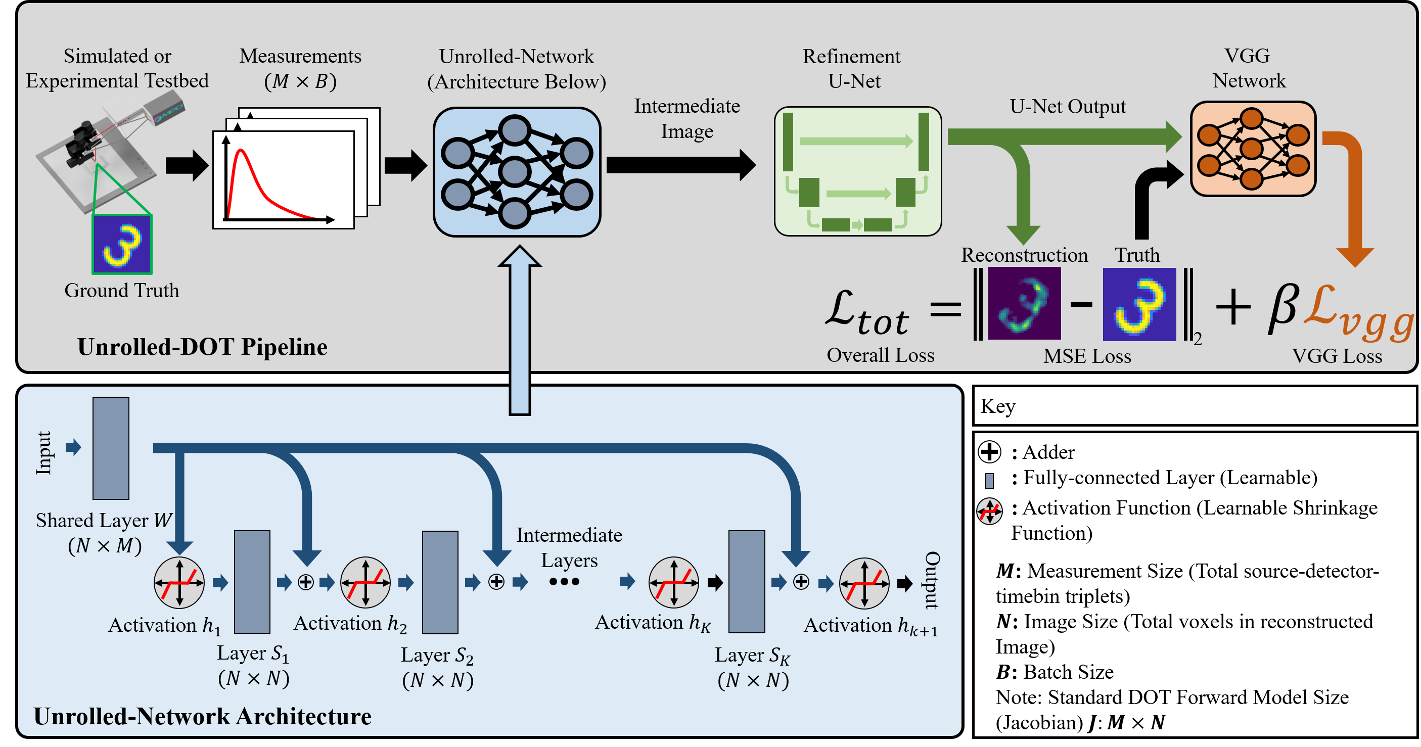
Official Implementation for Unrolled-DOT: an unrolled network for solving (time-of-flight) diffuse optical tomography inverse problems.
Yongyi Zhao, Ankit Raghuram, Fay Wang, Hyun Keol Kim, Andreas Hielscher, Jacob Robinson, and Ashok Veeraraghavan.
git clone https://github.com/yyiz/unrolled_DOT_code.git
cd unrolled_DOT_code
Before running the Unrolled-DOT package, please install the following:
- Python 3.6+
- MATLAB R2019b+
- Jupyter Lab
- Pytorch v1.9+
- Numpy v1.19+
- Matplotlib v3.3+
- Kornia v0.5.11
- parse
- scipy
- scikit-image
- h5py
- export_fig
- subaxis
The simulated datasets can be generated by running our code (see below). The real-world dataset is available at . The dataset consists of 5000 time-of-flight diffuse optical tomography measurements and their associated ground truth images, which were obtained from the MATLAB digits dataset. For more details please refer to our paper.
The files needed to run the code are:
5_29_21_src-det_10x10_scene_4cm/allTrainingDat_30-Sep-2021.mat
- In the file
unrolled_DOT_code/setpaths/paths.txt, set the four paths:libpath,datpath,resultpath,basepath. For example:
libpath = /path/to/libpath
datpath = /path/to/datpath
resultpath = /path/to/resultpath
basepath = /path/to/basepath
-
Place the datafiles in the following directories:
5_29_21_src-det_10x10_scene_4cm/: to be placed indatpathallTrainingDat_30-Sep-2021.mat: to be placed indatpath
-
Move the matlab packages
export_figandsubaxisto thelibpathpath
- The files referred to in this section can be found in the
basepath/fig4-5_recon_simdirectory. - Run the
RUNME_sim_unrolled_DOT.ipynbwith four configurations:unet_vgg_train_fashion_test_fashion.ini,train_fashion_test_fashion.ini,train_fashion_test_mnist.ini,train_mnist_test_mnist.ini, referring to training/testing the model on the fashion-MNIST dataset with a U-Net and VGG-loss, training/testing on the fashion-MNIST, training on the fashion-MNIST dataset and testing on MNIST, training/testing on the MNIST dataset without a U-Net and VGG-loss.- Re-run the script with each configuration, set the parameters by modifying the
confignamevariable to the corresponding.ini
- Re-run the script with each configuration, set the parameters by modifying the
- Run the
visReconSim.mscript to visualize the reconstructed test images with the trained model - The scripts for training the models found in the circular phantom reconstruction and simulated number-of-layers test can be found in
circ_RUNME_sim_unrolled_DOT.ipynbandtest_nlayers_sim.ipynb, respectively.
- The files referred to in this section can be found in the
basepath/fig12_recon_expdirectory. - Perform temporal filtering: in the
RUNME_gen_fig.mfile, run the code up to and including section 1. - Perform the training using the
unrolled-DOT_exp_train.ipynbscript. This file can be called using theRUNME_gen_fig.mscript (section 2) or directly run in a Jupyter notebook. The latter is better for monitoring training progress.unrolled-DOT_exp_train.ipynbreads a set of configuration file that sets the training parameters. The file is determined by setting theconfignamevariable to the desired file (a str) located in thefig12_recon_exp/settingsdirectory.tof_EML_dot_train_settings.iniand trains the network without the refinement U-Net and VGG-loss whileexp_vgg_unet.initrains the model with these components.
- Continue running sections 3-5 of
RUNME_gen_fig.m
Additional notes:
- Small differences with the results in the paper may occur due to non-deterministic behavior of the Pytorch-cuda training. However, these differences should be negligible.
- Labels are not included in the runtime vs MSE plot since these were labeled in latex to ensure updated references. Correct labels can be found by matching indices with the
label_arrvariable.
- To run this code, make sure you have generated the temporal-filtered data from section 1 of the real-world dataset training section. The files referred to in this section can be found in the
basepath/fig10_performance_analysisdirectory. - Run the
performance_analysis_train.ipynbscript.
After performing the steps above, the code for the other experiments in our paper can be run. Go into the folder for the desired experiment (in the basepath directory) and execute the associated matlab script.
This repository drew inspiration/help from the following resources:
- https://github.com/VITA-Group/ALISTA
- https://discuss.pytorch.org/t/how-can-i-make-the-lambda-trainable-in-softshrink-function/8733/2
- https://discuss.pytorch.org/t/encounter-the-runtimeerror-one-of-the-variables-needed-for-gradient-computation-has-been-modified-by-an-inplace-operation/836/26
- https://discuss.pytorch.org/t/runtimeerror-trying-to-backward-through-the-graph-a-second-time-but-the-buffers-have-already-been-freed-specify-retain-graph-true-when-calling-backward-the-first-time/6795
Refinement U-Net and VGG-Loss are based on example from FlatNet:
If you found our code or paper useful in your project, please cite:
@article{Zhao2023,
   author = {Yongyi Zhao and Ankit Raghuram and Fay Wang and Stephen Hyunkeol Kim and Andreas H. Hielscher and Jacob T. Robinson and Ashok Veeraraghavan},
   title = {{Unrolled-DOT: an interpretable deep network for diffuse optical tomography}},
   volume = {28},
   journal = {Journal of Biomedical Optics},
   number = {3},
   publisher = {SPIE},
   pages = {036002},
   year = {2023},
   doi = {10.1117/1.JBO.28.3.036002},
   URL = {https://doi.org/10.1117/1.JBO.28.3.036002}
}
If you have further questions, please email Yongyi Zhao at yongyi@rice.edu

