3D Teeth Reconstruction from CT Scans
This is the code for Computer Graphics course project in 2018 Fall to conduct 3D teeth reconstruction from CT scans, maintained by Kaiwen Zha and Han Xue.
Overview
3D Teeth Reconstruction from CT Scans
Dataset Annotation
Since our given dataset only contains raw CT scan images, we manually annotate the segmentations of 500 images using js-segment-annotator. You can download our dataset from here.
SegNet
We use SegNet as one of our base networks to conduct segmentation. We feed our annotated training data and train the network end-to-end, and evaluate it on our annotated testing data.
Dependencies
- Python 3.6
- TensorFlow 1.5.0
- Numpy
- Scipy
Preparation
- Download our pretrained models from here.
- Put the downloaded dataset /Images and /Labels into folder /Data/Training and /Data/Test.
- Put our pretrained models /Run_new into folder /Output.
Training Phase
- Run the training phase
python train.py- Start tensorboard in another terminal
tensorboard --logdir ./Output --port [port_id]Evaluating Phase
- Run the evaluating phase
python test.pyNote that you should have pretrained models /Run_new on folder /Output, and the predicted segmentations will be located in folder /Output/Run_new/Image_Output.
Qualitative Results
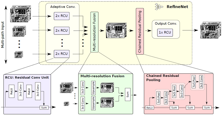
RefineNet
We also adopt RefineNet as our another base network to conduct segmentation. Here, we also use our annotated data to train and evaluate, and the code is finished by us from scratch, which implements with two interfaces for RefineNet and SESNet respectively.
Dependencies
-
Python 2.7
-
TensorFlow 1.8.0
-
Numpy
-
OpenCV
-
Pillow
-
Matplotlib
Preparation
- Download the checkpoint for ResNet backbone, TFRecords for training and testing data, generated color map, and our pretrained models from here.
- Put the downloaded dataset /images and /labels into folder /data.
- Put the ResNet checkpoint
resnet_v1_101.ckpt, color mapcolor_map, training and testing TFRecordstrain.tfrecordsandtest.tfrecordsinto folder /data. - Put our pretrained models into folder /checkpoints.
Training Phase
- If you have not downloaded the TFRecords, convert training and testing data into TFRecords by running
python convert_teeth_to_tfrecords.py- If you have not downloaded the color map, produce color map by running
python build_color_map.py- Run the training phase (enable multi-gpu training by tower loss)
python SESNet/multi_gpu_train.py --model_type refinenetNote that you can assign other command line parameters for training, like batch_size, learning_rate, gpu_list and so on.
Evaluating Phase
- Run the evaluating phase
python SESNet/test.py --model_type refinenet --result_path ref_resultNote that you should have trained models on folder /checkpoints, and the predicted segmentations will be located in folder /ref_result.
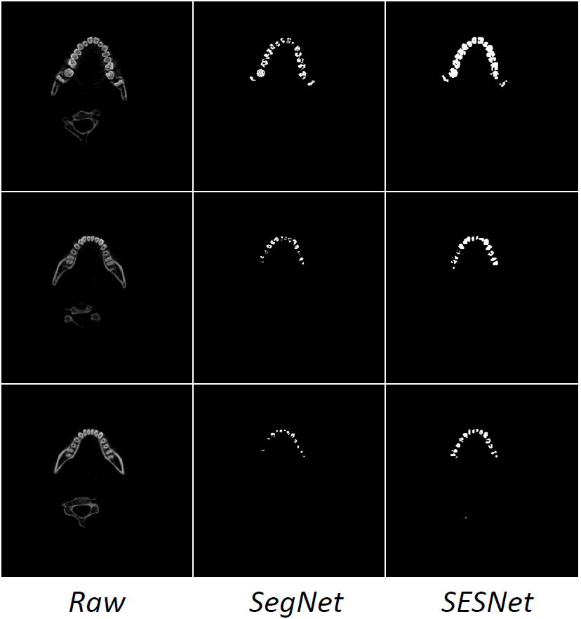
Qualitative Results
SESNet
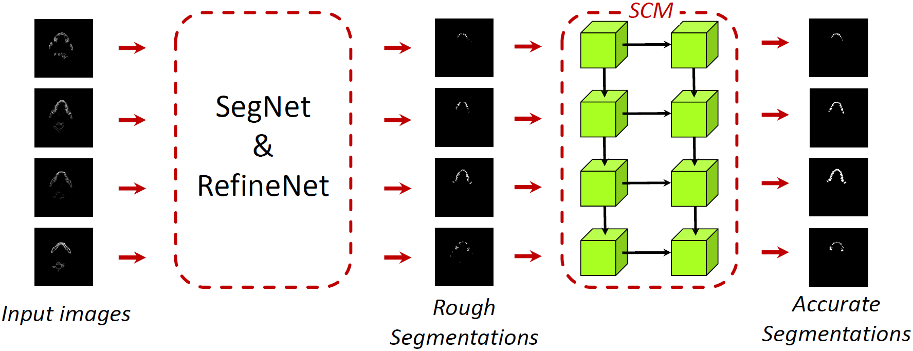
This architecture is proposed by us. First, we use base networks (SegNet or RefineNet) to predict rough segmentations. Then, use Shape Coherence Module (SCM), composed by 2-layer ConvLSTM, to learn the fluctuations of shapes to improve accuracy.
Dependencies
The same as the dependencies of RefineNet.
Preparation
The same as in RefineNet.
Training Phase
- Generate TFRecords for training and testing, and color map as in RefineNet does.
- Run the training phase (enable multi-gpu training by tower loss)
python SESNet/multi_gpu_train.py --model_type sesnetNote that you can assign other command line parameters for training as well, like batch_size, learning_rate, gpu_list and so on.
Evaluating Phase
- Run the evaluating phase
python SESNet/test.py --model_type sesnet --result_path ses_resultNote that you should have trained models on folder /checkpoints, and the predicted segmentations will be located in folder /ses_result.
Quantitative Results
| Pixel Accuracy | IoU | |
|---|---|---|
| SegNet | 92.6 | 71.2 |
| RefineNet | 99.6 | 78.3 |
| SESNet | 99.7 | 82.6 |
Qualitative Results
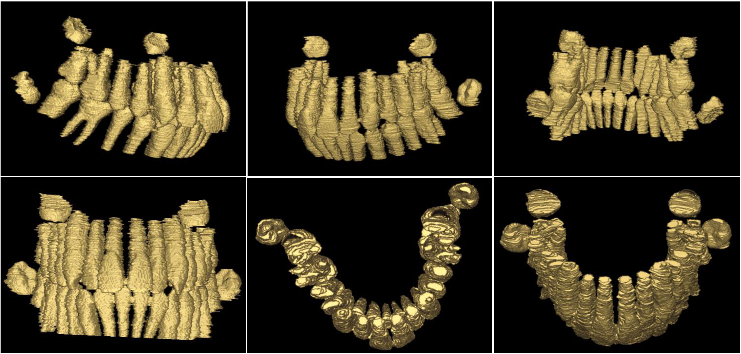
3D Reconstruction
Image Denoising
We use Morphology-based Smoothing by combining erosion and dilation operations.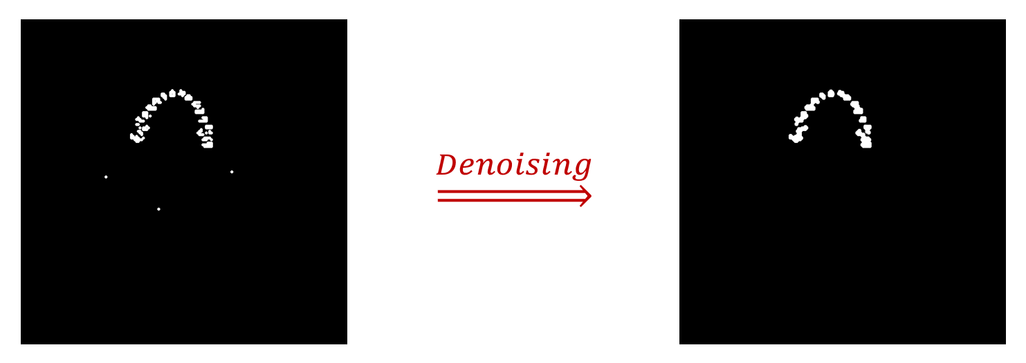
- We implemented it with MATLAB. Begin denoising by running
denoising(inputDir, outputDir, thresh);Note that inputDir is the folder for input PNG images, outputDir is the folder for output PNG images, and thresh is the threshold for binarizing (0~255).
Image Interpolation
In order to reduce the gaps between different layers, we use interpolation between 2D images to increase the depth of 3D volumetric intensity images.
- We implemented it with MATLAB. Begin interpolating by running
interpolate(inputDir, outputDir, new_depth, method)Note that inputDir is the folder for input PNG images, outputDir is the folder for output PNG images, new_depth is the new depth for 3-D volumetric intensity image, and method is the method for interpolation, which could be `linear', 'cubic', 'box', 'lanczos2' or 'lanczos3'.
- Convert continuous PNG files to RAW format (volume data) by running
python png2raw.py -in input_dir -out output_dir3D Visualization
We use surface rendering for 3D Visualization. We adopt Dual Marching Cubes algorithm to convert 3D volumetric intensity image into surface representation. This implementation requires C++11 and needs no other dependencies.
- To build the application and see the available options in a Linux environment type
$ make
$ ./dmc -help
A basic CMAKE file is provided as well.
- Extract a surface (OBJ format) from the volume type (RAW format) by running
$ ./dmc -raw FILE X Y ZNote that X, Y, Z are used to specify RAW file with dimensions.
- Display OBJ file by using software such as 3D Model Viewer or using our provided MATLAB function
obj_display(input_file_name);Demonstration
Contributors
This repo is maintained by Kaiwen Zha, and Han Xue.
Acknowledgement
Special thanks for the guidance of Prof. Bin Sheng and TA. Xiaoshuang Li.


