kalepy: Kernel Density Estimation and Sampling

This package performs KDE operations on multidimensional data to: 1) calculate estimated PDFs (probability distribution functions), and 2) resample new data from those PDFs.

Installation

from pypi (i.e. via pip)

pip install kalepy

from source (e.g. for development)

git clone https://github.com/lzkelley/kalepy.git
pip install -e kalepy/

In this case the package can easily be updated by changing into the source directory, pulling, and rebuilding:

cd kalepy
git pull
pip install -e .
# Optional: run unit tests (using the `nosetests` package)
nosetests

Basic Usage

import numpy as np
import matplotlib.pyplot as plt
import matplotlib as mpl

import kalepy as kale

from kalepy.plot import nbshow

Generate some random data, and its corresponding distribution function

NUM = int(1e4)
np.random.seed(12345)
_d1 = np.random.normal(4.0, 1.0, NUM)
_d2 = np.random.lognormal(0, 0.5, size=NUM)
data = np.concatenate([_d1, _d2])

xx = np.linspace(0.0, 7.0, 100)[1:]
yy = 0.5*np.exp(-(xx - 4.0)**2/2) / np.sqrt(2*np.pi)
yy += 0.5 * np.exp(-np.log(xx)**2/(2*0.5**2)) / (0.5*xx*np.sqrt(2*np.pi))

Plotting Smooth Distributions

# Reconstruct the probability-density based on the given data points.
# If `points` aren't provided then `kalepy` automatically generates them
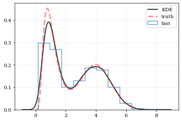
points, density = kale.density(data, probability=True)

# Plot the PDF
plt.plot(points, density, 'k-', lw=2.0, alpha=0.8, label='KDE')

# Plot the "true" PDF
plt.plot(xx, yy, 'r--', alpha=0.4, lw=3.0, label='truth')

# Plot the standard, histogram density estimate
plt.hist(data, density=True, histtype='step', lw=2.0, alpha=0.5, label='hist')

plt.legend()
nbshow()

Constructing statistically similar values

Draw a new sample of data-points from the KDE PDF

# Draw new samples from the KDE reconstructed PDF
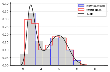
samples = kale.resample(data)

# Plot new samples
plt.hist(samples, density=True, alpha=0.5, label='new samples', color='0.65', edgecolor='b')


# Plot the KDE reconstructed PDF
plt.plot(points, density, 'k-', lw=2.0, alpha=0.8, label='KDE')
# Plot the "true" PDF
plt.plot(xx, yy, 'r--', alpha=0.4, lw=3.0, label='truth')

plt.legend()
nbshow()

Multivariate Distributions

# Load some random-ish data
data = kale.utils._random_data_3d_01()

# Construct a KDE
kde = kale.KDE(data)

import kalepy.plot

# Build a corner plot using the `kalepy` plotting submodule
corner = kale.plot.Corner(kde, figsize=[10, 10])

# Data points: red scatter and histograms
corner.plot_data(color='red', scatter=dict(s=10, alpha=0.15))

# KDE reconstructed density-distribution: blue contours and curves
corner.plot_kde(color='blue')


plt.show()

/Users/lzkelley/Programs/kalepy/kalepy/utils.py:1082: RuntimeWarning: covariance is not positive-semidefinite.
  data = np.random.multivariate_normal(np.zeros_like(sigma), cov, num).T

Fancy Usage

Reflecting Boundaries

What if the distributions you're trying to capture have edges in them, like in a uniform distribution between two bounds? Here, the KDE chooses 'reflection' locations based on the extrema of the given data.

# Uniform data (edges at -1 and +1)
np.random.seed(54321)
data = np.random.uniform(-1.0, 1.0, int(1e3))

# Histogram the data, use fixed bin-positions
edges = np.linspace(-1, 1, 12)
plt.hist(data, bins=edges, density=True, alpha=0.5, label='data', color='0.65', edgecolor='k')

# Standard KDE will undershoot just-inside the edges and overshoot outside edges
points, pdf_basic = kale.density(data, probability=True)
plt.plot(points, pdf_basic, 'r--', lw=4.0, alpha=0.5, label='Basic KDE')

# Reflecting KDE keeps probability within given bounds
points, pdf_basic = kale.density(data, reflect=True, probability=True)
plt.plot(points, pdf_basic, 'b-', lw=3.0, alpha=0.75, label='Reflecting KDE')

plt.legend()
nbshow()

Explicit reflection locations can also be provided (in any number of dimensions).

# Construct random data, add an artificial 'edge'
np.random.seed(5142)
edge = 1.0
data = np.random.lognormal(sigma=0.5, size=int(3e3))
data = data[data >= edge]

# Histogram the data, use fixed bin-positions
edges = np.linspace(edge, 4, 20)
plt.hist(data, bins=edges, density=True, alpha=0.5, label='data', color='0.65', edgecolor='k')

# Standard KDE with over & under estimates
points, pdf_basic = kale.density(data, probability=True)
plt.plot(points, pdf_basic, 'r--', lw=4.0, alpha=0.5, label='Basic KDE')

# Reflecting KDE setting the lower-boundary to the known value
#    There is no upper-boundary when `None` is given.
points, pdf_basic = kale.density(data, reflect=[edge, None], probability=True)
plt.plot(points, pdf_basic, 'b-', lw=3.0, alpha=0.5, label='Reflecting KDE')

plt.gca().set_xlim(edge - 0.5, 3)
plt.legend()
nbshow()

zhangyun-engineer/kalepy