ScType: Fully-automated and ultra-fast cell-type identification using specific marker combinations from single-cell transcriptomic data

Article: [https://doi.org/10.1038/s41467-022-28803-w]

ScType a computational method for automated selection of marker genes based merely on scRNA-seq data. The open-source portal (http://sctype.app) provides an interactive web-implementation of the method.

Quick start

# load libraries and functions
lapply(c("dplyr","Seurat","HGNChelper","openxlsx"), library, character.only = T)
source("https://raw.githubusercontent.com/IanevskiAleksandr/sc-type/master/R/gene_sets_prepare.R"); source("https://raw.githubusercontent.com/IanevskiAleksandr/sc-type/master/R/sctype_score_.R")

# get cell-type-specific gene sets from our in-built database (DB)
gs_list = gene_sets_prepare("https://raw.githubusercontent.com/IanevskiAleksandr/sc-type/master/ScTypeDB_short.xlsx", "Immune system") # e.g. Immune system, Liver, Pancreas, Kidney, Eye, Brain

# assign cell types
scRNAseqData = readRDS(gzcon(url('https://raw.githubusercontent.com/IanevskiAleksandr/sc-type/master/exampleData.RDS'))); #load example scRNA-seq matrix
es.max = sctype_score(scRNAseqData = scRNAseqData, scaled = TRUE, gs = gs_list$gs_positive, gs2 = gs_list$gs_negative)

# View results, cell-type by cell matrix. See the complete example below
View(es.max)

Cell type annotation example

Load and cluster the data

First let's load a PBMC 3k example dataset (see Seurat tutorial for more details on how to load the dataset using Seurat, https://satijalab.org/seurat/articles/pbmc3k_tutorial.html). The raw data can be found here.

# load libraries
lapply(c("dplyr","Seurat","HGNChelper"), library, character.only = T)

# Load the PBMC dataset
pbmc.data <- Read10X(data.dir = "./filtered_gene_bc_matrices/hg19/")
# Initialize the Seurat object with the raw (non-normalized data).
pbmc <- CreateSeuratObject(counts = pbmc.data, project = "pbmc3k", min.cells = 3, min.features = 200)

Next, let's normalize and cluster the data.

# normalize data
pbmc[["percent.mt"]] <- PercentageFeatureSet(pbmc, pattern = "^MT-")
# pbmc <- subset(pbmc, subset = nFeature_RNA > 200 & nFeature_RNA < 2500 & percent.mt < 5) # make some filtering based on QC metrics visualizations, see Seurat tutorial: https://satijalab.org/seurat/articles/pbmc3k_tutorial.html
pbmc <- NormalizeData(pbmc, normalization.method = "LogNormalize", scale.factor = 10000)
pbmc <- FindVariableFeatures(pbmc, selection.method = "vst", nfeatures = 2000)

# scale and run PCA
pbmc <- ScaleData(pbmc, features = rownames(pbmc))
pbmc <- RunPCA(pbmc, features = VariableFeatures(object = pbmc))

# Check number of PC components (we selected 10 PCs for downstream analysis, based on Elbow plot)
ElbowPlot(pbmc)

# cluster and visualize
pbmc <- FindNeighbors(pbmc, dims = 1:10)
pbmc <- FindClusters(pbmc, resolution = 0.8)
pbmc <- RunUMAP(pbmc, dims = 1:10)
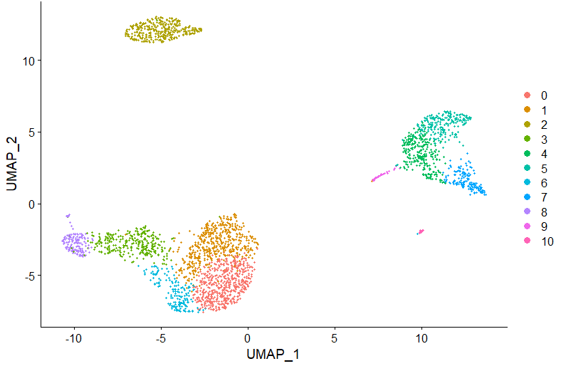
DimPlot(pbmc, reduction = "umap")

Cell type assignment

Now, let's automatically assign cell types using ScType. For that, we first load 2 additional ScType functions:

# load gene set preparation function
source("https://raw.githubusercontent.com/IanevskiAleksandr/sc-type/master/R/gene_sets_prepare.R")
# load cell type annotation function
source("https://raw.githubusercontent.com/IanevskiAleksandr/sc-type/master/R/sctype_score_.R")

Next, let's prepare gene sets from the input cell marker file. By default, we use our in-built cell marker DB, however, feel free to use your own data. Just prepare an input XLSX file in the same format as our DB file. DB file should contain four columns (tissueType - tissue type, cellName - cell type, geneSymbolmore1 - positive marker genes, geneSymbolmore2 - marker genes not expected to be expressed by a cell type)

In addition, provide a tissue type your data belongs to:

# DB file
db_ = "https://raw.githubusercontent.com/IanevskiAleksandr/sc-type/master/ScTypeDB_full.xlsx";
tissue = "Immune system" # e.g. Immune system,Pancreas,Liver,Eye,Kidney,Brain,Lung,Adrenal,Heart,Intestine,Muscle,Placenta,Spleen,Stomach,Thymus 

# prepare gene sets
gs_list = gene_sets_prepare(db_, tissue)

Finally, let's assign cell types to each cluster:

# get cell-type by cell matrix
es.max = sctype_score(scRNAseqData = pbmc[["RNA"]]@scale.data, scaled = TRUE, 
                      gs = gs_list$gs_positive, gs2 = gs_list$gs_negative) 

# NOTE: scRNAseqData parameter should correspond to your input scRNA-seq matrix. 
# In case Seurat is used, it is either pbmc[["RNA"]]@scale.data (default), pbmc[["SCT"]]@scale.data, in case sctransform is used for normalization,
# or pbmc[["integrated"]]@scale.data, in case a joint analysis of multiple single-cell datasets is performed.

# merge by cluster
cL_resutls = do.call("rbind", lapply(unique(pbmc@meta.data$seurat_clusters), function(cl){
    es.max.cl = sort(rowSums(es.max[ ,rownames(pbmc@meta.data[pbmc@meta.data$seurat_clusters==cl, ])]), decreasing = !0)
    head(data.frame(cluster = cl, type = names(es.max.cl), scores = es.max.cl, ncells = sum(pbmc@meta.data$seurat_clusters==cl)), 10)
}))
sctype_scores = cL_resutls %>% group_by(cluster) %>% top_n(n = 1, wt = scores)  

# set low-confident (low ScType score) clusters to "unknown"
sctype_scores$type[as.numeric(as.character(sctype_scores$scores)) < sctype_scores$ncells/4] = "Unknown"
print(sctype_scores[,1:3])

Please note that sctype_score function (used above) accepts both positive and negative markers through gs and gs2 arguments. In case, there are no negative markers (i.e. markers providing evidence against a cell being of specific cell type) just set gs2 argument to NULL (i.e. gs2 = NULL).

We can also overlay the identified cell types on UMAP plot:

pbmc@meta.data$customclassif = ""
for(j in unique(sctype_scores$cluster)){
  cl_type = sctype_scores[sctype_scores$cluster==j,]; 
  pbmc@meta.data$customclassif[pbmc@meta.data$seurat_clusters == j] = as.character(cl_type$type[1])
}

DimPlot(pbmc, reduction = "umap", label = TRUE, repel = TRUE, group.by = 'customclassif')

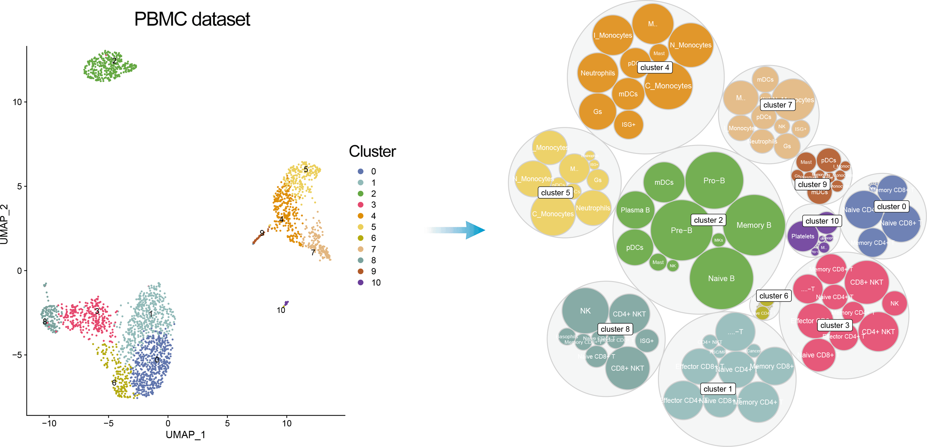
In addition, one can visualize a bubble plot showing all the cell types that were considered by ScType for cluster annotation. The outter (grey) bubbles correspond to each cluster (the bigger bubble, the more cells in the cluster), while the inner bubbles correspond to considered cell types for each cluster, with the biggest bubble corresponding to assigned cell type.

# load libraries
lapply(c("ggraph","igraph","tidyverse", "data.tree"), library, character.only = T)

# prepare edges
cL_resutls=cL_resutls[order(cL_resutls$cluster),]; edges = cL_resutls; edges$type = paste0(edges$type,"_",edges$cluster); edges$cluster = paste0("cluster ", edges$cluster); edges = edges[,c("cluster", "type")]; colnames(edges) = c("from", "to"); rownames(edges) <- NULL

# prepare nodes
nodes_lvl1 = sctype_scores[,c("cluster", "ncells")]; nodes_lvl1$cluster = paste0("cluster ", nodes_lvl1$cluster); nodes_lvl1$Colour = "#f1f1ef"; nodes_lvl1$ord = 1; nodes_lvl1$realname = nodes_lvl1$cluster; nodes_lvl1 = as.data.frame(nodes_lvl1); nodes_lvl2 = c(); 
ccolss= c("#5f75ae","#92bbb8","#64a841","#e5486e","#de8e06","#eccf5a","#b5aa0f","#e4b680","#7ba39d","#b15928","#ffff99", "#6a3d9a","#cab2d6","#ff7f00","#fdbf6f","#e31a1c","#fb9a99","#33a02c","#b2df8a","#1f78b4","#a6cee3")
for (i in 1:length(unique(cL_resutls$cluster))){
  dt_tmp = cL_resutls[cL_resutls$cluster == unique(cL_resutls$cluster)[i], ]; nodes_lvl2 = rbind(nodes_lvl2, data.frame(cluster = paste0(dt_tmp$type,"_",dt_tmp$cluster), ncells = dt_tmp$scores, Colour = ccolss[i], ord = 2, realname = dt_tmp$type))
}
nodes = rbind(nodes_lvl1, nodes_lvl2); nodes$ncells[nodes$ncells<1] = 1;
files_db = openxlsx::read.xlsx(db_)[,c("cellName","shortName")]; files_db = unique(files_db); nodes = merge(nodes, files_db, all.x = T, all.y = F, by.x = "realname", by.y = "cellName", sort = F)
nodes$shortName[is.na(nodes$shortName)] = nodes$realname[is.na(nodes$shortName)]; nodes = nodes[,c("cluster", "ncells", "Colour", "ord", "shortName", "realname")]

mygraph <- graph_from_data_frame(edges, vertices=nodes)

# Make the graph
gggr<- ggraph(mygraph, layout = 'circlepack', weight=I(ncells)) + 
  geom_node_circle(aes(filter=ord==1,fill=I("#F5F5F5"), colour=I("#D3D3D3")), alpha=0.9) + geom_node_circle(aes(filter=ord==2,fill=I(Colour), colour=I("#D3D3D3")), alpha=0.9) +
  theme_void() + geom_node_text(aes(filter=ord==2, label=shortName, colour=I("#ffffff"), fill="white", repel = !1, parse = T, size = I(log(ncells,25)*1.5)))+ geom_node_label(aes(filter=ord==1,  label=shortName, colour=I("#000000"), size = I(3), fill="white", parse = T), repel = !0, segment.linetype="dotted")
  
scater::multiplot(DimPlot(pbmc, reduction = "umap", label = TRUE, repel = TRUE, cols = ccolss), gggr, cols = 2)

sessionInfo();
[1] HGNChelper_0.8.1        SeuratObject_4.0.2      Seurat_4.0.3     dplyr_1.0.6

Automatically detect a tissue type of the dataset

In addition, if the tissue type of the input dataset is unknown, ScType provides a functionality for automated guessing of a tissue type.

# load auto-detection function
source("https://raw.githubusercontent.com/IanevskiAleksandr/sc-type/master/R/auto_detect_tissue_type.R")
db_ = "https://raw.githubusercontent.com/IanevskiAleksandr/sc-type/master/ScTypeDB_full.xlsx";

# guess a tissue type
tissue_guess = auto_detect_tissue_type(path_to_db_file = db_, seuratObject = pbmc, scaled = TRUE, assay = "RNA")  # if saled = TRUE, make sure the data is scaled, as seuratObject[[assay]]@scale.data is used. If you just created a Seurat object, without any scaling and normalization, set scaled = FALSE, seuratObject[[assay]]@counts will be used

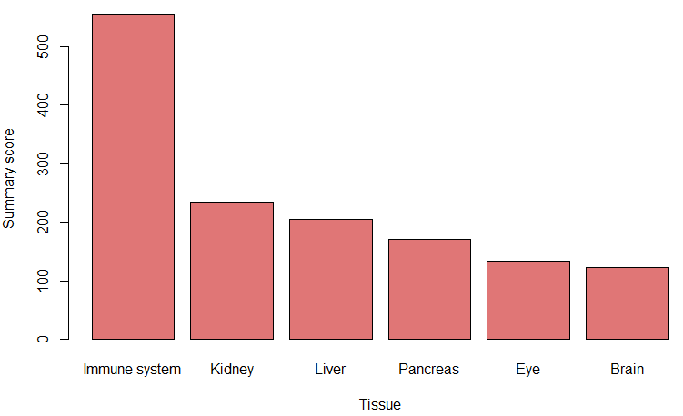
The highest summary score represents the most probable tissue type.

Contact information

For any questions please contact Aleksandr Ianevski (aleksandr.ianevski@helsinki.fi)

zhanxw/sc-type