The goal of project is applying PCA to data visualization and image reconstruction. The project builds the applications of PCA and extends it in Matlab. Meanwhile, the implementations are tested on datasets.
Basically, there are 2 ways to implement PCA, which are derived from covariance matrix and Singular Value Decomposition (SVD). For a given data set d*N (d>>N), the SVD overcomes the implication of covariance matrix that the latter is computatinally expensive (ie., d is the number of dimensionally while N is that of sample).
Below presents 5 steps to build PCA:
1. Data Centralization
2. Eigenanalysis/SVD process
3. Finding principal components
4. Encoding data point
5. Reconstructing data point
Let's dive into the functions implementing 2 versions of PCA in Matlab.
- pca1.m      % PCA based on covariance matrix
- pca2.m      % PCA based on Singular Value Decomposition (SVD)
- data_vis.m  % visualize iris dataset on computed principal components
- img_rec.m   % reconstruct images from digit dataset using SVD-PCA
- KPCA.m      % implements Kernel PCA to reduce dimensionality, referred to prof. Deng Cai @ZJU
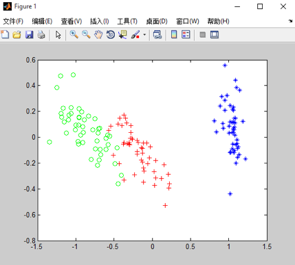
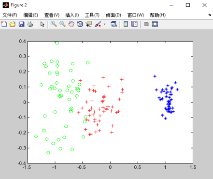
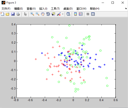
Then follows the resultant images got from the applications. The data visualization is concerned about projecting iris data on main principal components, by which we can compare the significance of each eigenvector.

Figure 1, projection of iris data on PC1-PC2.

Figure 2, projection of iris data on PC1-PC3.

Figure 3, projection of iris data on PC2-PC3.
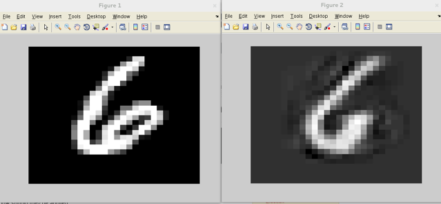
The digits are reconstructed by using SVD-PCA, which chooses principal components with probability of variance (PoV) being larger than 90%. In my case, the number of choosen components is 47, on which the reconstructed digits are based.

Figure 4, original digit (left) and its reconstructed digit (right).