`gtsummary`

The gtsummary package for R produces beautiful, customizable, publication-ready tables to summarize statistical models. Results from several models are presented side-by-side, with uncertainty estimates in parentheses (or brackets) underneath coefficient estimates.

Here are a few benefits of gtsummary over some alternative packages:

html, rtf, and LaTeX output
Excellent integration with:
- RStudio: When users type gtsummary(models), the summary table immediately appears in RStudio's Viewer window.
- knitr: Dynamic document generation FTW.
- Designed from the ground up with the tidy paradigm in mind.
Endlessly customizable tables, thanks to the power of the gt package.
- In the next section of this README, you will find tables with colored cells, weird text, spanning column labels, row groups, titles and subtitles, footnotes, significance stars, etc.
gtsummary uses the broom package to extract information from model objects. This means that gtsummary supports dozens of model types out of the box. Most importantly, broom already has a large community of users, and whenever broom improves, gtsummary improves.
By using the broom and gt package for key operations, gtsummary has a massively simplified codebase. This should improve long term code maintainability, and allow contributors to participate through GitHub.
gtsummary is developed with unit tests.

Installation

The gt and gtsummary packages are not available on CRAN yet. You can install them from github:

library(remotes)
remotes::install_github('rstudio/gt')
remotes::install_github('vincentarelbundock/gtsummary')

Make sure you also install tidyverse, as gtsummary depends on a lot of its packages (e.g., stringr, dplyr, tidyr, purrr):

install.packages('tidyverse')

Using gtsummary

Preliminaries

Load packages and download some data from the RDatasets repository. Then, estimate 5 different models and store them in a named list. The name of each model in that list will be used as a column label:

library(gt)
library(MASS)
library(gtsummary)
url <- 'https://vincentarelbundock.github.io/Rdatasets/csv/HistData/Guerry.csv'
dat <- read.csv(url) 
dat$Clergy <- ifelse(dat$Clergy > 40, 1, 0) # binary variable for logit model

models <- list()
models[['OLS 1']] <- lm(Literacy ~ Crime_prop + Infants, dat)
models[['NBin 1']] <- glm.nb(Literacy ~ Crime_prop + Donations, dat)
models[['OLS 2']] <- lm(Desertion ~ Crime_prop + Infants, dat)
models[['NBin 2']] <- glm.nb(Desertion ~ Crime_prop + Donations, dat)
models[['Logit 1']] <- glm(Clergy ~ Crime_prop + Infants, dat, family = binomial())

Simple table

Produce a simple table.

gtsummary(models)

RStudio will render this automatically as an html table. If you do not use RStudio, read the next section to learn how to save to file.

Of course, gtsummary can also summarize single models:

mod <- lm(Clergy ~ Crime_prop, data = dat)
gtsummary(mod)

Output formats

To save a table to file, use the filename argument. gtsummary guesses the output format based on the filename extension. The supported extensions are: .tex, .rtf, .html (ASCII/Text tables coming soon).

gtsummary(models, filename = 'table.tex')
gtsummary(models, filename = 'table.rtf')
gtsummary(models, filename = 'table.html')

If filename is not specified, gtsummary returns a gt object which can be further customized and rendered by the relevant functions in the gt package, such as as_raw_html, as_latex, or as_rtf. RStudio renders the html version of this object automatically.

SE, t, p, CI

gtsummary prints an uncertainty estimate in parentheses below the corresponding coefficient estimate. The statistic argument must be a string which is equal to conf.int or to one of the columns produced by the broom::tidy function. When using conf.int, users can specify a confidence level with the conf_level argument.

gtsummary(models, statistic = 'std.error')
gtsummary(models, statistic = 'p.value')
gtsummary(models, statistic = 'statistic')
gtsummary(models, statistic = 'conf.int', conf_level = .99)

Titles and subtitles

You can add titles and subtitles to your table as follows:

gtsummary(models, 
          title = 'This is a title for my table.',
          subtitle = 'And this is the subtitle.')

Notes

Add notes to the bottom of your table:

gtsummary(models, 
          notes = list('Text of the first note.', 
                       'Text of the second note.'))

Rename, reorder, and subset coefficients

The coef_map argument is a named vector which allows users to rename, reorder, and subset coefficient estimates. Values of this vector correspond to the "clean" variable name. Names of this vector correspond to the "raw" variable name. The table will be sorted in the order in which terms are presented in coef_map. Coefficients which are not included in coef_map will be excluded from the table.

cm <- c('Crime_prop' = 'Crime / Population',
        'Donations' = 'Donations',
        '(Intercept)' = 'Constant')
gtsummary(models, coef_map = cm)

An alternative mechanism to subset coefficients is to use the coef_omit argument. This string is a regular expression which will be fed to stringr::str_detect to detect the variable names which should be excluded from the table.

gtsummary(models, coef_omit = 'Intercept|Donation')

Rename, reorder, and subset goodness-of-fit statistics

gof_omit is a regular expression which will be fed to stringr::str_detect to detect the names of the statistics which should be excluded from the table.

gtsummary(models, gof_omit = 'DF|Deviance')

Column groups (spanning labels)

Create spanning labels to group models (columns):

gtsummary(models) %>%
       gt::tab_spanner(label = 'Literacy', columns = c('OLS 1', 'NBin 1')) %>%
       gt::tab_spanner(label = 'Desertion', columns = c('OLS 2', 'NBin 2')) %>%
       gt::tab_spanner(label = 'Clergy', columns = 'Logit 1')

Stars: Statistical significance markers

Some people like to add "stars" to their model summary tables to mark statistical significance. The stars argument can take three types of input:

NULL omits any stars or special marks (default)
TRUE uses these default values: * p < 0.1, ** p < 0.05, *** p < 0.01
Named numeric vector for custom stars.

gtsummary(models)
gtsummary(models, stars = TRUE) 
gtsummary(models, stars = c('+' = .1, '*' = .01))

Digits, rounding, exponential notation

The fmt argument defines how numeric values are rounded and presented in the table. This argument follows the sprintf C-library standard. For example,

%.3f will keep 3 digits after the decimal point, including trailing zeros.
%.5f will keep 5 digits after the decimal point, including trailing zeros.
Changing the f for an e will use the exponential decimal representation.

Most users will just modify the 3 in %.3f, but this is a very powerful system, and all users are encouraged to read the details: ?sprintf

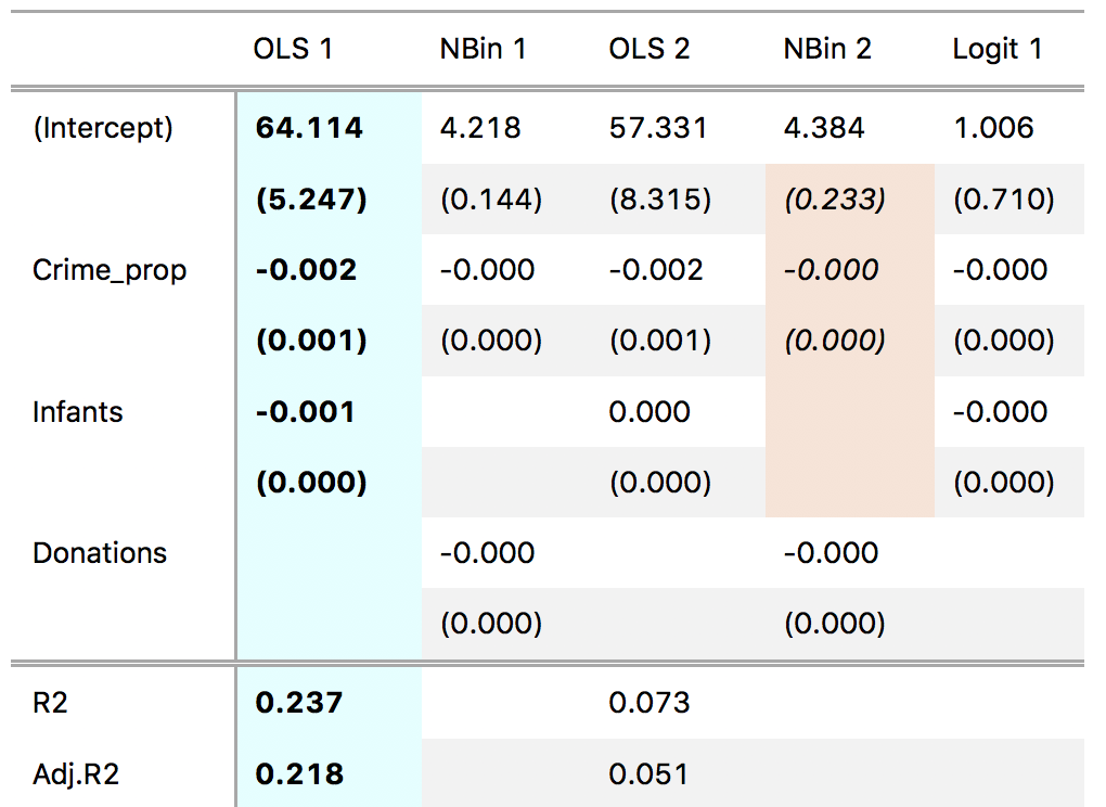
gtsummary(models, fmt = '%.7f')

Styles and colors

The power of the gt package makes gtsummary tables endlessly customizable. For instance, we can color columns and cells, and present values in bold or italics:

gtsummary(models) %>%
    tab_style(style = cells_styles(bkgd_color = "lightcyan",
                                   text_weight = "bold"),
              locations = cells_data(columns = vars(`OLS 1`))) %>%
    tab_style(style = cells_styles(bkgd_color = "#F9E3D6",
                                   text_style = "italic"),
              locations = cells_data(columns = vars(`NBin 2`),
                                     rows = 2:6))

Fancy text with markdown: bold, italics, etc.

Thanks to gt, gtsummary accepts markdown indications for emphasis and more:

gtsummary(models, 
          title = md('This is a **bolded series of words.**'),
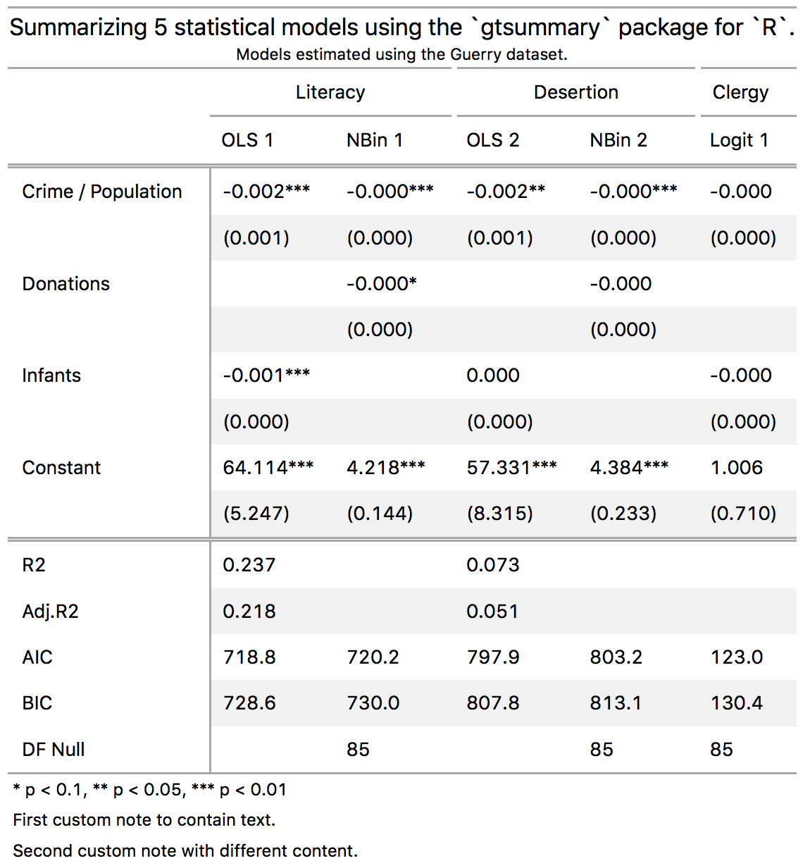
          notes = list(md('And an *emphasized note*.')))

Complex table

This is the code I used to generate the "complex" table posted at the top of this README.

cm <- c('Crime_prop' = 'Crime / Population',
        'Donations' = 'Donations',
        'Infants' = 'Infants',
        '(Intercept)' = 'Constant')
gtsummary(models,
          coef_map = cm,
          stars = TRUE,
          gof_omit = "Statistics|^p$|Deviance|Resid|Sigma|Log.Lik|^DF$",
          title = 'Summarizing 5 statistical models using the `gtsummary` package for `R`.',
          subtitle = 'Models estimated using the Guerry dataset.',
          notes = c('First custom note to contain text.',
                    'Second custom note with different content.')) %>%
    # add spanning labels
    gt::tab_spanner(label = 'Literacy', columns = c('OLS 1', 'NBin 1')) %>%
    gt::tab_spanner(label = 'Desertion', columns = c('OLS 2', 'NBin 2')) %>%
    gt::tab_spanner(label = 'Clergy', columns = 'Logit 1')

Power users

The gt package allows a bunch more customization and styling. Power users can use gtsummary's extract function to produce a tibble which can easily be fed into gt.

> gtsummary::extract(models)
# A tibble: 21 x 8
   group     term        statistic `OLS 1` `NBin 1` `OLS 2` `NBin 2` `Logit 1`
   <chr>     <chr>       <chr>     <chr>   <chr>    <chr>   <chr>    <chr>
 1 estimates (Intercept) estimate  64.114  4.218    57.331  4.384    1.006
 2 estimates (Intercept) statistic (5.247) (0.144)  (8.315) (0.233)  (0.710)
 3 estimates Crime_prop  estimate  -0.002  -0.000   -0.002  -0.000   -0.000
 4 estimates Crime_prop  statistic (0.001) (0.000)  (0.001) (0.000)  (0.000)
 5 estimates Infants     estimate  -0.001  ""       0.000   ""       -0.000
 6 estimates Infants     statistic (0.000) ""       (0.000) ""       (0.000)
 7 estimates Donations   estimate  ""      -0.000   ""      -0.000   ""
 8 estimates Donations   statistic ""      (0.000)  ""      (0.000)  ""
 9 gof       R2          ""        0.237   ""       0.073   ""       ""
10 gof       Adj.R2      ""        0.218   ""       0.051   ""       ""
# … with 11 more rows

Alternative summary table packages for R

There are several excellent alternative summary table packages for R:

zhaoxiaohe/gtsummary