Welcome to the PyGran webpage!
PyGran is an open-source toolkit primarily designed for analyzing DEM simulation data. In addition to performing basic and custom post-processing, PyGran enables running DEM simulation with LIGGGHTS in Python. It's recommended to use PyGran with Python 3.7 and later versions.
The main features of PyGran:
- Interactive DEM simulation and/or analysis using Python
- Parallel "multiple parameter, single script" simulation for parametrization and sensitivity analysis
- Intuitive (matlab-like) syntax for particle manipulation and analysis (e.g. slicing, concatenating, etc.)
- Post-processing coupled particle-mesh DEM simulation with VTK
- Quick and easy plotting of DEM data with matplotlib
- Support for high-performance computing with MPI
The core modules in PyGran are:
- simulation: provides APIs for running DEM simulation
- analysis: provides methods and algorithms for post-processing DEM data
- params: defines material properties
If your find PyGran useful in your research, please consider citing the following paper:
@article{aam2019pygran,
  title={PyGran: An object-oriented library for DEM simulation and analysis},
  author={Abi-Mansour, Andrew},
  journal={SoftwareX},
  volume={9},
  pages={168--174},
  year={2019},
  publisher={Elsevier},
  doi={10.1016/j.softx.2019.01.016}
}
Quick Installation
Installing PyGran is quite straight forward on a Unix/Unix-like machine. Just fire up a terminal and then use pip (or pip3) to install PyGran:
pip install PyGran --userFor more options and information on setting up PyGran on Ubuntu 18.04 (LTS), see the installation page.
Basic Usage
Running DEM simulation with LIGGGHTS
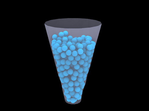
PyGran also provides an interface for running DEM simulation with LIGGGHTS. This is achieved by importing the simulation module as shown in the script below for simulating granular flow in a hopper.
from PyGran import simulation
from PyGran import params

# Create a DEM parameter dictionary
param = {

	'boundary': ('f','f','f'),
	'box':  (-1e-3, 1e-3, -1e-3, 1e-3, 0, 4e-3),

	'species': (
                    {'material': params.stearicAcid, 'radius': ('constant', 5e-5)},
		   ),

	'gravity': (9.81, 0, 0, -1),

	'mesh': {
                 'hopper': {'file': 'silo.stl', 'mtype': 'mesh/surface',
		 'material': params.steel},
                },
}

# Instantiate a DEM class
sim = simulation.DEM(**param)

# Insert 1000 particles for species 1 (stearic acid)
insert = sim.insert(species=1, value=1000)

# Evolve the system in time
sim.run(nsteps=1e6, dt=1e-7)
Post-processing DEM output data
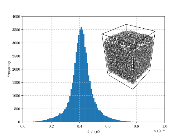
Using PyGran for doing post-analysis is also quite straight forward. Computing particle overlaps shown below for instance can be done in few lines of code:
from PyGran import analysis

# Instantiate a System class from a dump file
Gran = analysis.System(Particles='granular.dump')

# Instantiate a nearest-neighbors class
NNS = analysis.Neighbors(Particles=Gran.Particles)
overlaps = NNS.overlaps
For more examples on using PyGran for running DEM simulation, check out the examples page.


