LiDAR Compensation 🚨

This repository contains the source code of the LiDAR Compensation.

Getting Started 🚀

These instructions will get you a copy of the project up and running on your local machine for development and testing purposes.

Prerequisites 📋

Robot Operating System (ROS) needs to be installed (link) and a rosbag with raw data is needed.

ros-kinetic-desktop-full

Installing 🔧

The folders given are ROS packages that need to be inside your workspace following this structure:

your-ws
  build
  devel
  src
    lidar-compensation
       imgs
       include
       launch
       ...

Then, the steps are:

Create workspace and src folder

mkdir your-ws
cd your-ws
mkdir src
catkin_make

Clone the repository inside src

cd src
git clone git@serv-driverless-33:david.alvarez/lidar-compensation.git

Compile the code (it may take some time the first time)

cd ..
catkin_make

Running the algorithm with raw data ️

Launch the nodelet

source devel/setup.bash
roslaunch lidar-compensation LidarCompensation.launch

Then, the nodelet is waiting for the input data.

Play the rosbag:

cd <folder_with_rosbags>
rosrun rqt_bag rqt_bag rosbag_name.bag

and publish the velodyne_points topic.

cd <folder_with_rosbags>
rosbag play rosbag_name.bag --loop

and all the topics in the rosbags will be published. The nodelet should start computing and printing results.

Visualization 🔮

Use RVIZ to visualize the point cloud and the markers published with the cones detected:

rviz &

and add type of data PointCloud2 and MarkerArray.

Understanding the code 💡

The main purpose of this code is to compensate the distortion that appears in the data received from the LiDAR due to the movement of the car. This happens because the LiDAR takes non-zero time for completing a turn. Therefore, since information is return for each full turn, position will be distorted due to the car movement.

At slow (car) speeds this effect is not noticeable, however at higher speeds correcting this distortion can be crucial for a correct perception of the surrounding environment.

For fixing ideas, let’s suppose that the LiDAR is rotating at a frequency of 10Hz and that the car is going (in a straight line) at 25m/s (90km/h). Then, there may be points such that the detection time differs by 0.1s (i.e. a period). Therefore, by this time the car will have moved (and the LiDAR with it) 2.5m (0.1s * 25m/s). This is the actual (maximum) distortion.

Get velocity from IMU 🌪

We get the (linear) velocity of the car at that moment from a IMU.

geometry_msgs::Vector3 velocity = odom->twist.twist.linear;

Last angle of vision 📐

Obviously, there is not such a thing like the distortion of a complete PointCloud, since it will be different for each point. This distortion depends on the time between the recording of the last point and the current one. This elapsed time is proportional to the difference of angles between points, therefore we will work with angles since they can be more easily computed.

We need to work with the last angle, and not with first angle because the LiDAR assign the time stamp of this last point to the whole PointCloud.

The last angle of vision θEnd is computed as follows:

pcl::PointXYZ& pointEnd = cloud.points[cloud.points.size() - 1];
float thetaEnd = atan(-pointEnd.y, pointEnd.x);

Actual compensation 📝

For compensating a PointCloud we iterate on points and for each point we do the following.

Compute it’s angle θ: same as previous section computation.
Compute the differences in angles (known θ and θEnd):

float deltaTheta = theta - thetaEnd;
  if (deltaTheta < 0)
    deltaTheta += 2 * M_PI;

Compute elapsed time (known the LiDAR frequency and the difference between angles):

float time = deltaTheta / ( 2 * M_PI * FREQUENCY );

Compensate point (known elapsed time and linear velocity of the car):

point.x -= time * velocity.x;
point.y -= time * velocity.y;
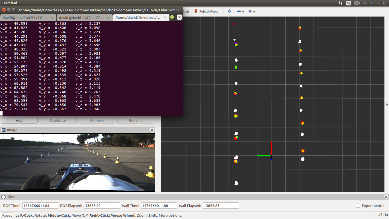
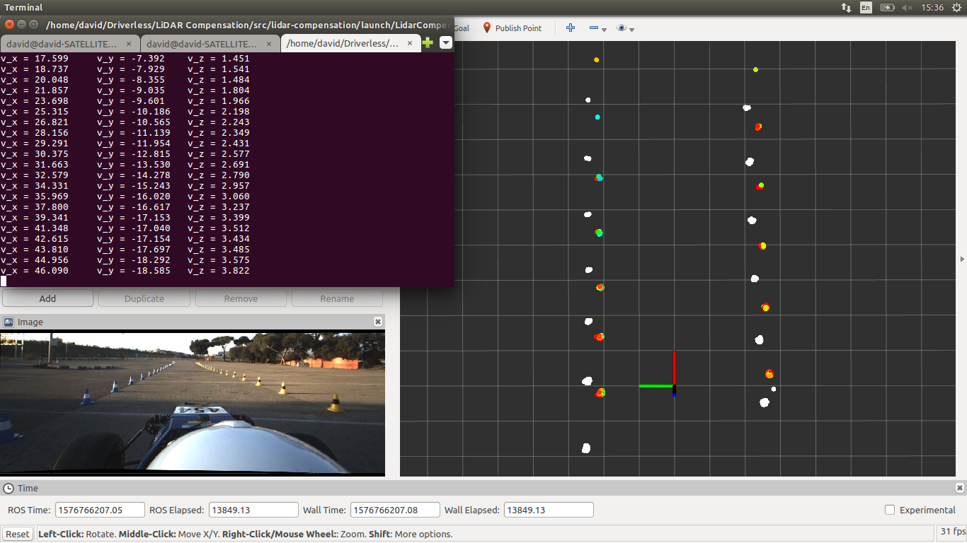
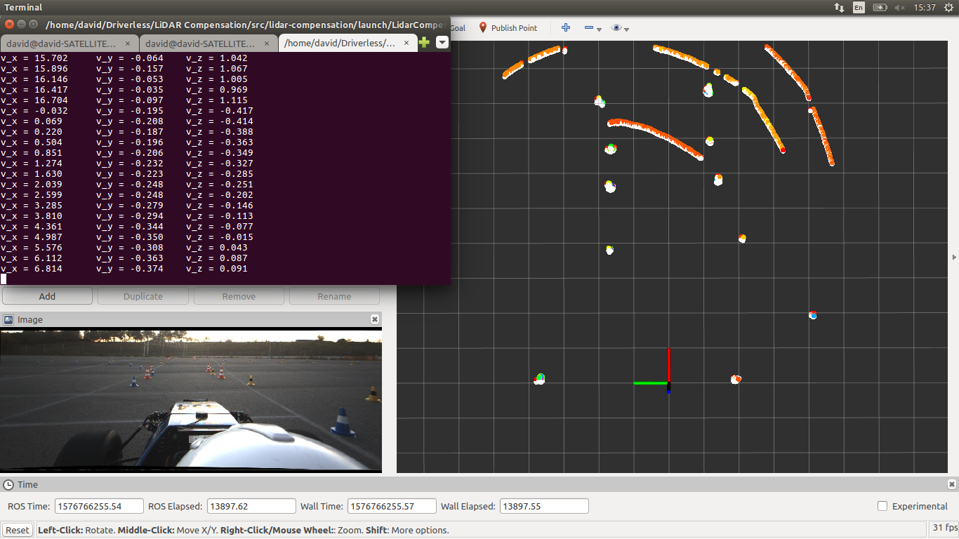
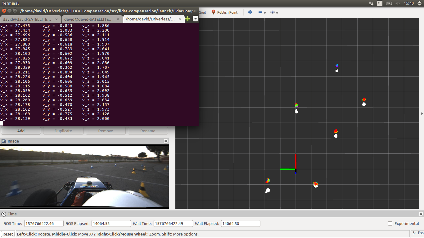
point.z -= time * velocity.z;

Results 🎯

We will know present some examples of the compensation code in operation. In all the examples below the linear velocity of the car is shown in the open terminal in the top left corner (in km/h). The LiDAR frequency in all this examples is fixed and set to 10Hz. In the images are shown both the non-compensated filter PointCloud and the compensated:

Non-compensated: colored points.
Compensated: white points.

Acceleration ⬆

This is an (straight) acceleration test at a moderate speed (around 35km/h).

As you can see the compensation works as expected. The cones are being “pushed forward” always (as it should be) and cones pairs line up.

Faster acceleration ⬆

Here is another example of an (straight) acceleration test at a higher speed (around 75km/h) and with a larger field of vision.

One thing to note is that the first left cone is “alone” because the distortion is large enough not to see it’s partner.

Lateral compensation in acceleration ↗

This is also another example of an (straight) acceleration test, but in this case the car is not centered on the track and it’s turning right to center it.

We can see here the lateral compensation (more accentuated in the cones on the left).

No compensation - Slow speed 🐌

Here is an example in which the car is going at a slow speed (around 4km/h).

As we can see there is no appreciable compensation, as expected.

Curved road 🔄

Finally, an example of compensation on a curved road.

Non deformed shapes 💎

As a last detail, we show a side view of the PointCloud where we can see that the shapes are not being deformed while compensating.

Difficulties 🛠

Ask a Perception member ;)

Authors ✒️

David Álvarez Rosa

zhuhaijun753/lidar-compensation