Optimizing Sparse Matrix Kernels

⚓ Introduction
⚒️ Setup
📜 Usage
📚 Approach
📈 Experiment Evaluation
☑️ Retrospective
✏️ Reference

⚓ Introduction

Myriads of applications hinge on sparse matrix operations, such as computer networks, social graph, 3D visualization, PageRank, integer factorization, machine learning, etc. However, they also tend to be computationally heavy and resource thirsty. As the size and complexity of those problems grows, efficient processing for sparse linear algebra operations on many-core systems is urgently needed.

lsolver is a basic infrastructure developed to optimize the performance of the sparse matrix triangular solve.

The structure of the project is as follows.

.
├── data
|   ├── matrices    // Put datasets here.
|   ├── out         // Results of lower triangular solve.
|   └── stat        // Raw data of the experiments.
├── include
│   ├── mm_io.h
│   ├── parallel.h  // Parallel implementations.
│   ├── serial.h    // Serial implementations.
│   ├── util.h
│   ├── verify.h    // Result verification algorithm.
│   └── wrapper.h   // Wrapper functions for external libs.
├── lib             // External libraries.
├── obj             // Compliled binary files.
├── src
│   ├── parallel.cpp
│   ├── plot.py     // Script for plotting experiment data.
│   ├── run.cpp     // Project entry.
│   ├── serial.cpp
│   ├── util.cpp
│   └── verify.cpp
└── test
    ├── test1.cpp   // Test on trivial1.
    ├── test2.cpp   // Test on trivial2.
    ├── test3.cpp   // Test on torso1.
    ├── test4.cpp   // Test on TSOPF_RS_b678_c2.
    ├── test5.cpp   // Test on torso1 (parallel).
    └── test6.cpp   // Test on TSOPF_RS_b678_c2 (parallel).

⚒️ Setup

Environment

The current development is on Linux (Debian). Use gcc-10 to complie the source code. Two external libraries, MM_IO and Seldon are used to handle part of the I/O operations.

ℹ️ Please see ./include/wrapper.h for integration details.

Build

Run the following commands to build this project.

git clone -j8 repository-url

(cd lib && sh mm_io.sh) && make all

Use the following if you have built it once.

make rebuild

You can directly pack the code by runing the following.

make dist

Test cases

Download the two matrices TSOPF_RS_b678_c2 and torso1. Place the under the .\data\matrices folder together with their b-matrices.

Note that matrices have to be in the Matrix Market format.

ℹ️ Please see the example files in .\data\trivial.

(The *_tri.mtx files are corresponding lower triangular matrices. They are not required as this infrastructure will generate them when processing their original matrices.)

📜 Usage

Execution

Run the following commands to execute lsolver.

make lsolver

./lsover ./path/to/L-matrix ./path/to/b-matrix

You can check the correctness of the results by adding the compiler flag TEST.

make CFLAGS=-DTEST lsolver

The verification algorithm will be introduced in the following sections.

ℹ️ Please see the ./src/verfy.cpp for details.

Testing

To invoke all tests in one go, use

make testall

To run a single test case, use

make run_test[%d]

To build a single test case, use

make test[%d]

📚 Approach

There are many ways to solve a sparse lower triangular system. This project implements three simple methods, namely, naive, guarded and graph.

ℹ️ Please see ./src/serial.cpp and ./src/parallel for implementation details.

The `naive`

The naive algorithm is nothing but a simple forward method that solves the system by traversing all columns and subsequently subtracting them from the b-matrix. In this way, the value of the top diagonal element v_i on the fringe at each iteration equates is the value of x_i. The time complexity of this algorithm is bounded by O(|b|+f+n) (which is asymptotically O(f+n)), where b is the size of the b-matrix and f is the number of FLOPs (floating-point operations).

The `guarded`

The guarded is a modified version of the naive algorithm. The nuance is that the computation at each iteration is “guarded” by a zero check for the element of the b-matrix. When the element of the b-matrix is 0 at that moment, then subtracting its products with the current column from the b-matrix makes will make no actual contribution to the result. This will significantly reduce the #FLOPs in the computation.

However, the theoretical complexity of the guarded method is still along the lines of O(f+n) since it still needs to walk through each element to check 0’s. This is by no means ideal because when matrices are huge (which is often the case), the time complexity is governed by n as opposed to the outer loop.

The `graph`

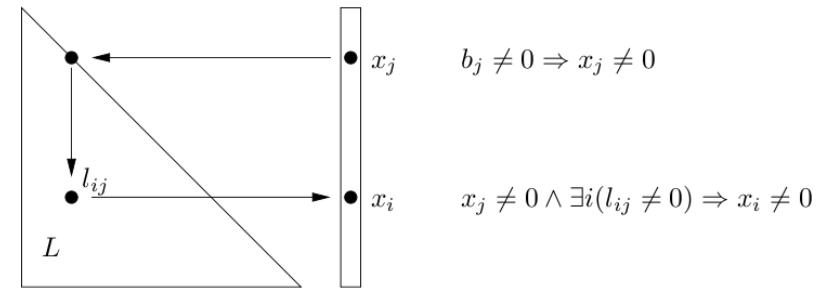
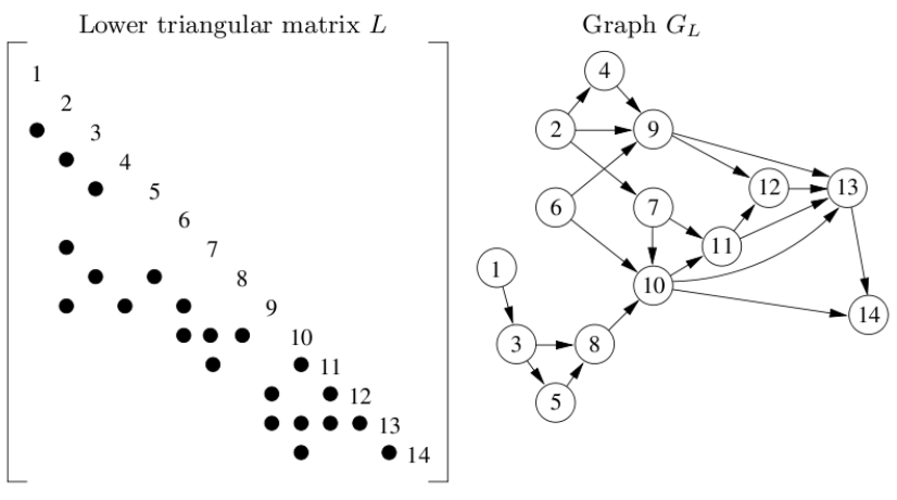
The graph is a novel up-looking [1], direct approach [3] that exploits the sparsity of the linear system before solving it. It employs the fundamental DFS (depth-first search) algorithm to explore the nonzero-pattern of the b-matrix prior to the computation of the linear system. In layman’s term, we can know which of the elements in the b-matrix are zero without actually looping through it. This tackles the dominant factor n which, in turn, makes the theoretical time complexity O(|b|+f).

N.B. the definition of “zero” here is a bit subtle. It does not mean the value zero(0) but the zero notion without the need of any computation [2], i.e. (3 - 3) is non-zero here.

Result verification

The verification algorithm takes the lower triangular matrix, the b-matrix and the computed result as inputs and produces a boolean value as output. It takes advantage of the Compressed sparse column (CSC) format. It first traverses the matrix column by column. Then it computes and accumulates the product with the corresponding x in the results along the way. After finishing the iterations, it compares the accumulated values of each column with that of the b-matrix to verify the results.

The fault tolerance value (TOL) of the current implementation is 10^12.

ℹ️ Please see ./src/verify.cpp for implementation details.

📈 Experiment Evaluation

FLOPs

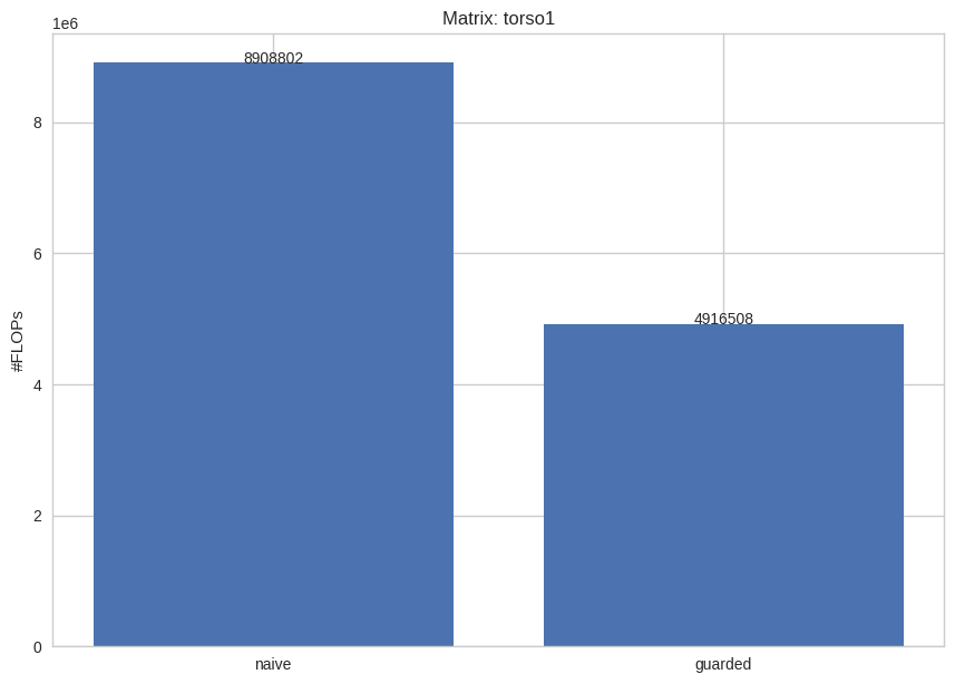
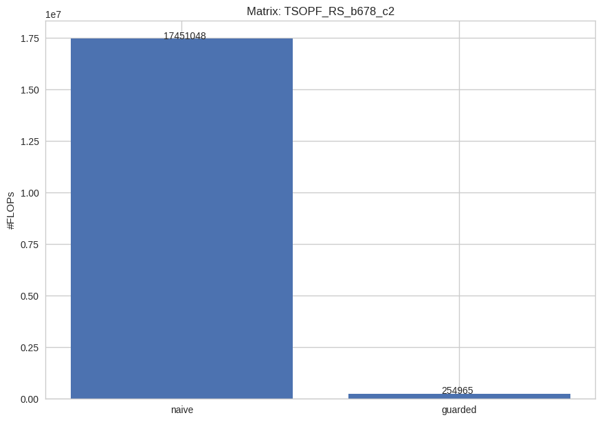
Firstly, I compared the naive method with the guarded method on the number of FLOPs needed for solving the lower triangular system. From the below bar charts, we can see that the guarded method dramatically reduces the number of FLOPs. Thus, the more sparse the matrices are, the more efficient this method should be.

Serial optimization

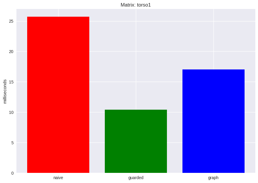
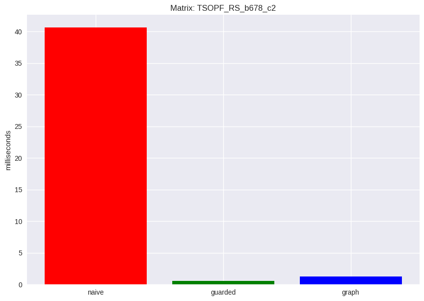
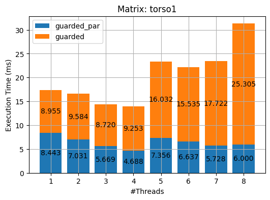
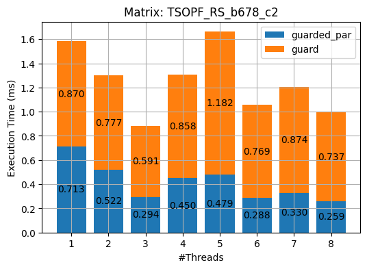
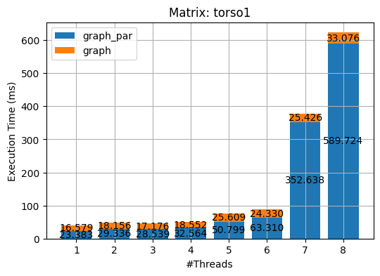
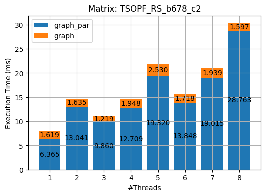
I benchmarked the execution time of the three algorithms on the two matrices. Surprisingly, the simple guarded method outperforms both the naive and the innovative graph approach by a significantly large margin. This could well be the case that my implementation of the graph algorithm is not quite efficient, and further experiments are needed.

Note that I have not yet implement the full version of the graph algorithm specified in [2]. A fully-fledged graph algorithm employs a pruned matrix tree, the etree [1]. The etree not only preserves the scarcity of the matrix but also embodies the dependencies of the entries of the graph in topological order.

ℹ️ Please see [1] for theory background and ./src/serial.cpp for implementation details.

Parallel optimization

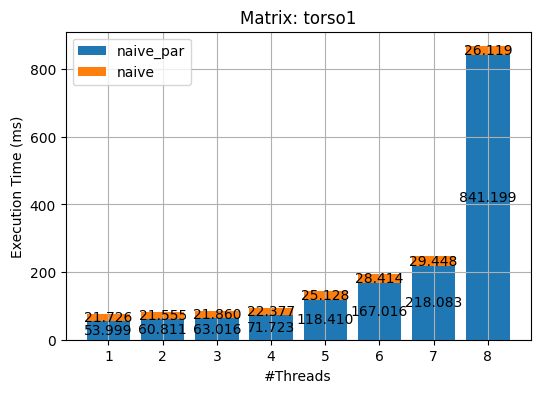
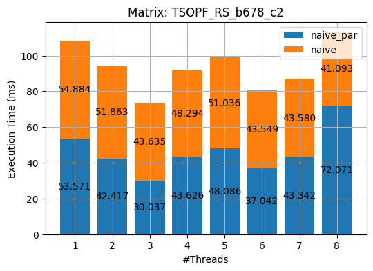
I used OpenMP to parallel the aforementioned three methods. The results of the experiments on the 2 matrices are shown in the following plots. (_par stands for the parallel implementations of the corresponding algorithm.)

⚠️ All the the following experiments are conducted on my laptop, which is a bit “powerless”. My computer has 1 socket in total and 4 cores per chip. Each chip has 2 CPU units, i.e. each of them can run 2 threads in parallel. That is to say, the machine can only truly parallel a maximum of 8 threads. That's why the benchmarking is capped by 8 threads.

ℹ️ To run experiences for parallel implementations, use the following command, and replace the N with the number of threads needed.

export OMP_NUM_THREADS=N && make run_test[%d]

As we can see from the above figures, almost all parallel implementations incurred overhead except the guarded_par. I deem it is due to the following three reasons

I did not rewrite the serial programs to fit the OpenMP constructs but rather made as minimal changes as possible.
The paralleled portions of the serial programs are not computationally heavy. That is the overhead of multithreading, e.g. creating, queueing and managing threads, cancelled or even overshadowed the small benefits that the parallelism brings about.
Again, my implementations could be improved :)

ℹ️ Please see the./src/plot.py for scripting details and ./src/parallel.cpp for implementation details.

☑️ Retrospective

The current version of this project has developed a simple infrastructure that enables batch testing and experiments on solving lower triangular linear systems.
Three algorithms, namely, the naive, the guarded and the graph, have been implemented. Correctness is guaranteed.
The most striking fact to me is that how efficient a straightforward solution can be as the guarded approach, albeit simple, stands out. I believe that in nowadays research, reviewing or revitalizing simple methods could be powerful.
As mentioned in the Serial optimization subsection, the graph algorithm has not been fully developed. The etree and the node order, if implemented, should be able to boost the performance of graph [4].
The benchmark of the same algorithm differs on different linear systems it deals with. => Workload is indeed one of the Rate Holes of performance analysis [5].
From the experiment results, we can see clearly that resource contention happened during the benchmarking as the performance of the none parallel methods fluctuated greatly in accordance with that of their parallel implementations. Better isolated experiments should be conducted in the future.
One of the pitfalls of my experiments is that no meaningful performance metrics were adopted in the evaluation.
Again, the parallel implementations could be improved by rewriting the three algorithms with OpenMP.
Later, I will host the project directly in a local clusters to overcome the “eight-thread barrier”.

✏️ Reference

[1] Davis, T.A. et al., "A survey of direct methods for sparse linear systems," Acta Numer'16.

[2] Davis, "A Direct methods for sparse linear systems," SIAM 2006.

[3] Cheshmi, Kazem et al., "ParSy: Inspection and transformation of sparse matrix computations for parallelism," SC'18.

[4] Cheshmi, Kazem et al., "NASOQ: numerically accurate sparsity-oriented QP solver," TOG'20.

[5] Jain, "The art of computer systems performance analysis, techniques for experimental design, measurement, simulation and modeling." 1992.

ziyuhuang123/lsolver

Optimizing Sparse Matrix Kernels

Table of contents

⚓ Introduction

⚒️ Setup

Environment

Build

Test cases

📜 Usage

Execution

Testing

📚 Approach

The `naive`

The `guarded`

The `graph`

Result verification

📈 Experiment Evaluation

FLOPs

Serial optimization

Parallel optimization

☑️ Retrospective

✏️ Reference

ziyuhuang123/lsolver

Optimizing Sparse Matrix Kernels

Table of contents

⚓ Introduction

⚒️ Setup

Environment

Build

Test cases

📜 Usage

Execution

Testing

📚 Approach

The naive

The guarded

The graph

Result verification

📈 Experiment Evaluation

FLOPs

Serial optimization

Parallel optimization

☑️ Retrospective

✏️ Reference

The `naive`

The `guarded`

The `graph`