For this assignment, I decided to focus on the model computational performance. Specifically, I implemented the assignment also in Rust to see what the performance gain will be. The reasons are that (1) I want to learn Rust but every class is Python + PyTorch, and (2) current NLP research is all done by prototyping in Python, yet there is a virtue in the experience of programming usable deployable and fast solutions. Note: I don't want to be mean to Python; it certainly has its place and advantages.
I understand that the task was to program this in Python, which I hope I fulfilled. Yet I also hope that you will find this comparison interesting.
The Rust code is twice as large* and took much longer to complete. *Running grep -r -E "^\s*[{}]\s*$" rust/src/ | wc -l reveals that more than 100 lines are just opening or closing brackets, so the code size is not that significant. Also, strong typing allows for more finer tooling. An example would be clippy, which helped me discover multiple bad design patterns.
data/                  # not supplied, paste the files here for reproducibility
 - de-{eval,train}.tt
 - de-test.t
data_measured/
 - {r,p}-de-eval{,-smooth}.tt # model outputs
 - time-{1,2,3}        # measured results for graphs
 - time-{1,2,3}.png    # exported graphs
meta/                  # scripts for measuring performance and accuracy
 - graph.py            # produce graphs given logs time-{1,2,3} in data_measured
 - run_times.py        # measure performance from r-build-time and p-run-time recipes
 - eval.py             # computes metrics and prints table
rust/                  # Rust source code
python/                # Python source code
Makefile               # Makefile for common recipes
make r-print-eval trains three models on the data and outputs the CONLL-U file to data_measured/p-de-eval{,-smooth,-vanilla}.tt, similarly make r-print-eval produces data_measured/r-de-eval{,-smooth}.tt (assuming stable Rust compiler in path). The semantics of the rest of the command line arguments is intuitive from the Makefile: print_acc self-reports the accuracy on anything it computes (comp_test, comp_train or comp_eval). smooth enables emission smoothing, no_normalize disables layer normalization.
File paths are relative and hardcoded because there are no plans to make this portable and there were already too many switches. Both versions assume that they are run from the top-level directory (the directory the README.md is in). If print_pred is present, the program outputs predictions to stdout. Progress is output to stderr.
Even though the Viterbi algorithm should be mostly deterministic, there is an issue with number representation and rounding. There appears to be a difference in accuracy based on the underlying numeric type used (f32 vs f64).
Unseen tokens were dealt with by substituting the emission probability with 1, thus relying on the surrounding transition probabilities.
I tried to use the same algorithmic steps in both solutions so that they are comparable. It is, however, still possible, that I mistakenly used some other data structure, assuming it was the same. The two versions produce almost the same outputs (they differ slightly in the smoothed version).
Another solution to the issue of storing very small probabilities would be to work in log space. One of the issues is that it no longer supports the computation of cumulative probability (because the probabilities there are summed). It did not however affect the model performance and for simplicity reasons I left it out.
Lowercasing the input led to decrease in train and eval accuracy by 0.57% and 0.16%.
Words which represented numbers could be stemmed into one group by the following processing:
tok = tok.strip('.')
if re.match('\d+.?', tok):
    tok = '<DIGIT>'
This resulted in train and eval accuracy of 97.30% and 91.23%.
Trellis layer normalization (so that it sums up to 1) had no effect on the output, but still can be turned off by no_normalize. It would have an effect in case of longer sentences. Making the normalization to sum to something other than 1 did not affect the accuracy.
Structures in both versions follow the same naming scheme. The programs function as follows:
- Train
Loaderis created, which also creates aMapperobjects (see Note) - HMM Model parameters are estimated from the training data.
- Eval or Test
Loaderis created, reusing TrainingMapper. - Based on the arguments, datasets are evaluated (
comp_test,comp_trainorcomp_eval).
The HMM class contains code for initialization and Viterbi and can be used generically. HMMTag inherits from this class and adds specific functions for initialization from Loader and evaluation. Both implementations start with main.{rs,py}.
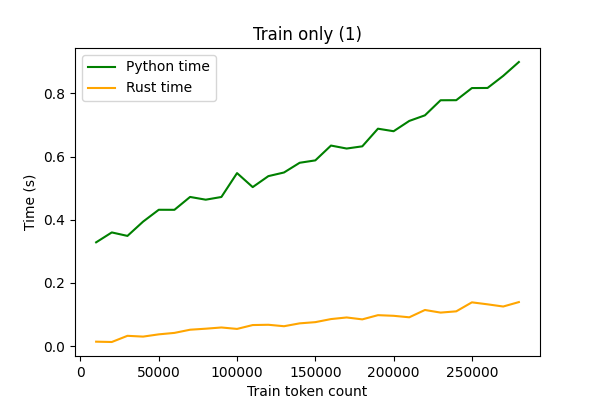
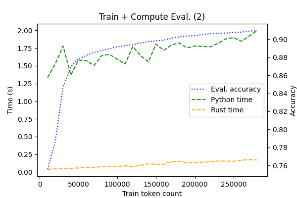
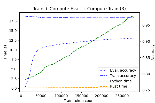
The performance was measured with respect to changing training data size (steps of 10000 tokens). The task was (1) train, (2) train + evaluate on eval, (3) train + evaluate on train and eval. Accuracy of these models was also measured. The measured times are without writing to files. Rust version is compiled with the --release flag and Python is run with -O. Both versions use aforementioned smoothing.
Figure 1 shows simply that in training, the Rust implementation seems to be faster by the factor of ~6.
Figure 2 also shows that the Rust implementation is more stable (possibly because of the lack of runtime). We also see that there seems to be diminishing return in performance after we pass 50k train tokens. Python ends at 2.00s and Rust on 0.17s (factor of ~12).
Evaluating the whole data proved to be the most challenging task. This is shown in Figure 3. While Python ends at 18.81s, for Rust it is 0.29s (factor of ~65). Train accuracy is 97.43%, evaluation accuracy 90.96%. The training accuracy is decreasing because the capacity of the model is getting shared with a larger amount of examples.
A good question would be, why does the running time not increasy hyperlinearly, as the complexity suggests? An answer would be that the complexity is hyperlinear with respect to the state space and not observation count in total.
I did not try to especially optimize algorithmic performance. For example, the trellis is allocated and cleared for every sentence in the data. This could be done much more efficiently by creating one static one (the size of the longest sentence) and reusing that for the computation. It does not need to be cleared, because every cell is first written to and only then read.
One of the biggest performance boosts was gained by creating a hashmap mapping from string (both for words and for tags), convert everything to numbers (Rust version uses 8bytes, which is unnecessary), manipulate just these numbers and only when printing revert back. This is done by the Loader and Mapper classes in both versions.
Also, both versions contain code for computing sequence observation probability in trellis (sum instead of max), but is turned off in both versions. The Rust version gets an unfair advantage in this because it is removed compile-time, while in Python, the interpreter has a bit more work to do.
I also experimented with rudimentary smoothing. This is done in the HMMTag class by adding fractional counts to emission probabilities, so that there are no hard zeroes. I had however only a slight effect on the model performance (only accuracy difference was for training data). Smoothing other parameters does not make much sense and also had no effect.
The Rust code also contains the toy ice-cream X weather example. It can be run from the rust directory with cargo test -- --nocapture.
This is an idea beyond the scope of this homework, but I would nevertheless like to see it implemented (and especially to see the performance) or any comments that show the caveats of this approach.
In order to better handle unknown word handling, all tokens could be split into subword units, e.g. by Byte Pair Encoding. This would allow the splitting to be trained not only on annotated data but also on unannotated. The HMM parameters could be then estimated as follows:
Assume the sequence SENT A-B C-B (BPE compound A-B at the beginning of the sentence, followed by C-B). Since individual subwords have the same POS tags, the starting and transition probabilities can be computed in an almost normal way: both A and B are starting and both A, B are followed by C, D (4 transitions). Furthermore, emission probabilities can also remain unchanged. This is counterintuitive because it will lead to affixes with POS tags as the same word (e.g. un-do-able -> (un, ADJ), (do, ADJ), (able, ADJ).) To avoid this, I would suggest early stopping of the BPE algorithm.
Further assume, that we trained two sets of HMM parameters: in the standard way (E, T, P) and also with subword units (E', T', P'). The main difference would be in inference. If the next token to be processed is present in the training data, the standard parameters and approach would be used. If it is, however, not in the training data, it is split to subwords: c = A1-A2-..-An. The starting and transition probability would be estimated from P' and T'. Emission probability would then be the average of the parameters for individual subwords: E''(c, s) = [E'(A1, s)+E'(A2, s)+..+E'(An, s)]/n.
The emission probability function can be extended to convex interpolate between the standard and subword version: E'''(c, s) = a * E''(c, s) + (1-a) * E(UNK, s). Here a is a parameter, which can be estimated from held-out data.
Completely another approach would be some sort of sensitive stemming, which would remove affixes that do not change the part of speech. This would reduce the amount of word forms while preserving correctness in the annotation.
This sections lists results of models in descending order. The file eval.py is included, because I changed it to produce markable tables.
Highest results from {r,p}-eval-smooth.tt, accuracy: 90.96%.
| Tag | Prec. | Recall | F1 |
|---|---|---|---|
DET |
0.8220 | 0.9768 | 0.8927 |
NOUN |
0.9307 | 0.9139 | 0.9222 |
VERB |
0.9202 | 0.9211 | 0.9206 |
ADP |
0.9343 | 0.9775 | 0.9554 |
. |
0.9608 | 1.0000 | 0.9800 |
CONJ |
0.9513 | 0.8974 | 0.9236 |
PRON |
0.8679 | 0.8364 | 0.8519 |
ADV |
0.9043 | 0.8051 | 0.8518 |
ADJ |
0.8088 | 0.7213 | 0.7625 |
NUM |
0.9906 | 0.7778 | 0.8714 |
PRT |
0.8685 | 0.9251 | 0.8959 |
X |
0.2222 | 0.0909 | 0.1290 |
File {r,p}-eval.tt, accuracy: 90.95%.
| Tag | Prec. | Recall | F1 |
|---|---|---|---|
DET |
0.8232 | 0.9755 | 0.8929 |
NOUN |
0.9296 | 0.9141 | 0.9218 |
VERB |
0.9202 | 0.9211 | 0.9206 |
ADP |
0.9348 | 0.9775 | 0.9557 |
. |
0.9608 | 1.0000 | 0.9800 |
CONJ |
0.9498 | 0.8974 | 0.9228 |
PRON |
0.8671 | 0.8364 | 0.8515 |
ADV |
0.9043 | 0.8058 | 0.8523 |
ADJ |
0.8099 | 0.7222 | 0.7635 |
NUM |
0.9905 | 0.7704 | 0.8667 |
PRT |
0.8712 | 0.9251 | 0.8973 |
X |
0.2222 | 0.0909 | 0.1290 |
I did not provide any comment for the alpha=0.9 parameter in matplotlib function call in graph.py, because that seems just absurd and commenting every other line reduces readability.


