| Documentation | Build Status | License |
|---|---|---|
 |
 |
OceanTurb.jl provides software for solving one-dimensional
models that approximate the physics of the
ocean's turbulent surface boundary layer.
Open julia, press ] to enter package manager mode, and type
pkg> add OceanTurbWith OceanTurb.jl installed, try
using OceanTurb

@use_pyplot_utils # add utilities for plotting OceanTurb Fields

     N = 128        # Model resolution
     H = 128        # Vertical extent of the model domain
    Qb = 1e-7       # Surface buoyancy flux (positive implies cooling)
  dTdz = 1e-3       # Interior/initial temperature gradient
    Δt = 10minute   # Time step size
tfinal = 8hour      # Final time

# Build the model with a Backward Euler timestepper
model = KPP.Model(N=N, H=H, stepper=:BackwardEuler)

# Set initial condition
T₀(z) = 20 + dTdz * z
model.solution.T = T₀

# Set boundary conditions
model.bcs.T.top = FluxBoundaryCondition(Qb / (model.constants.α * model.constants.g))
model.bcs.T.bottom = GradientBoundaryCondition(dTdz)

# Run the model
run_until!(model, Δt, tfinal)

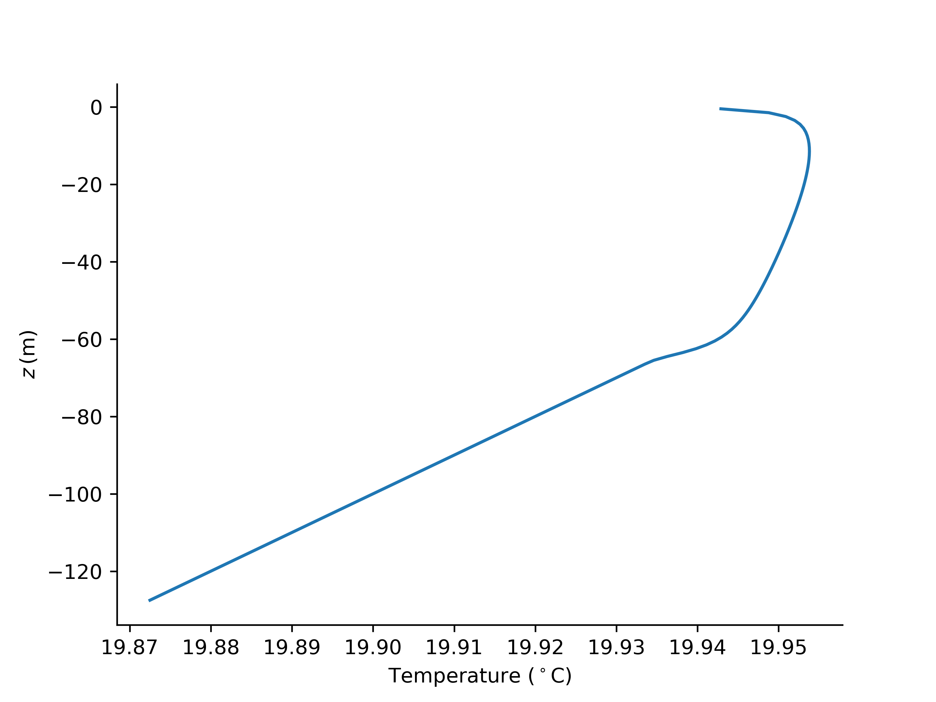
plot(model.solution.T)
removespines("top", "right")
xlabel("Temperature (\$ {}^\\circ \\mathrm{C} \$)")
ylabel(L"z \, \mathrm{(m)}")
to make a plot that looks something like this:
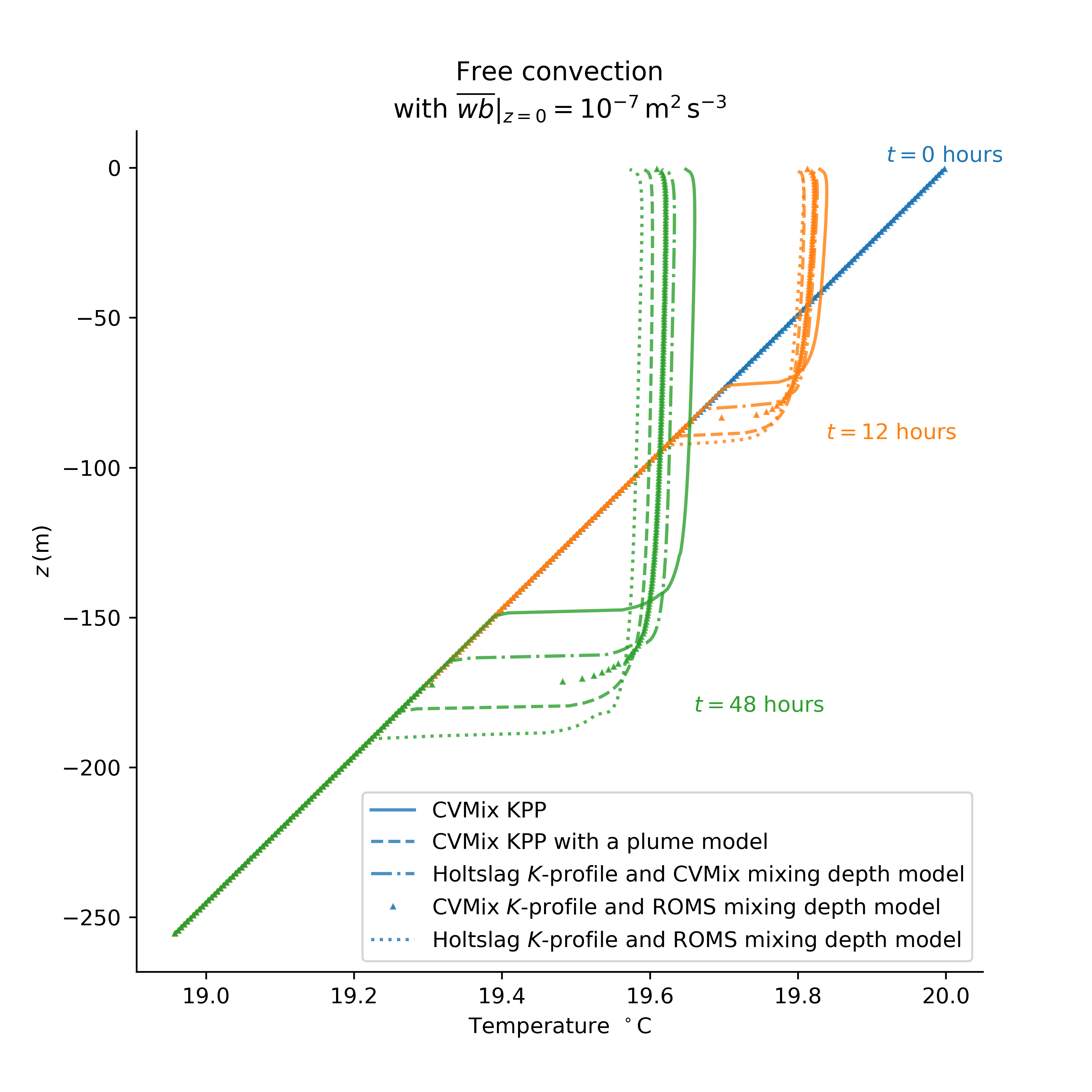
For a more complicated example, see examples/modular_kpp_example.jl
to produce
which compares various flavors of the 'KPP' boundary layer model with one another.
Check the documentation or src/models/ for the latest update
on turbulence models we have implemented.

