Overview

This document outlines a proposed approach for setting interim population goals for declining species. We seek to develop SMART interim population goals:

Specific: What needs to be accomplished? Who is responsible for it? What steps need to be taken to achieve it?
Measurable: Goals are stated in quantitative terms and based on indicators that are tracked through routine monitoring.
Achievable: Goals represent population recovery scenarios that would occur through sustained but incremental investment in conservation. The goals also recognize that fully recovering species that have experienced long-term declines is unrealistic in many cases.
Relevant: How do these goals relate to CWS/ECCC/GOC mandates?
Time-bound: The time horizon represents the scale at which conservation action has the potential to achieve goals.

For each species that has experienced long-term population declines, we construct two projection curves that represent alternative future pathways populations could take:

population declines continue at the same mean annual rate as in the past, or
populations achieve a specified target population growth at a specified point in the future, resulting in a “recovery curve”

As new monitoring data is collected in the future, progress towards recovery can be measured by compared the observed population trajectory to the projections.

Method description & case study

A stand-alone script to run these analyses is provided as projection.R. The remainder of this document explains the rationale and steps within that script in more detail.

Historical trajectory and population trend

We start by fitting a population model to monitoring data for a focal species. We accomplish this using the bbsBayes2 R package for species monitored by the North American Breeding Bird Survey. We fit the ‘gamye’ version of the model, which uses hierarchical splines to model curvilinear population trajectories, as well as random annual year effects.

The code below fits the model for Clay-colored Sparrow:

# Focal species
species_name <- "Clay-colored Sparrow"

# Species names and abbreviations (avian core 2022)
ac <- read_xlsx("data/1_Avian_Core_20220422_FULLVERSION.xlsx")

# 4 letter species abbreviation code
sp_code <- subset(ac, English_Name == species_name)$Species_ID

# Directory where fitted model will be stored 
filename <- paste0("fitted_models/",sp_code,".RDS")

# Fit model for this species, save resulting indices
if (!file.exists(filename)){
  
  # Stratify data
  s <- stratify(by = "bbs_usgs", species = species_name)
  
  p <- tryCatch(expr = {prepare_data(s)},
                error = function(e){NULL})
  
  # Fit model & generate indices
  if (is.null(p)) next
  p <- prepare_data(s)
  md <- prepare_model(p, model = "gamye")
  m <- run_model(md, save_model = FALSE)
  i <- generate_indices(model_output = m, regions = "country")
  
  # National indices
  samps <- i$samples$country_Canada
  
  # Save results
  sp_results <- list(samps = samps)
  saveRDS(sp_results, file = filename)
}

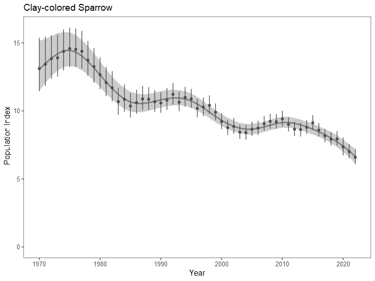
Below, we plot the annual population indices for the species:

Population projections

For each species, we construct projections of hypothetical trajectories that represent optimistic but potentially achievable scenarios of population recovery. The projections begin with the current rate of long-term population decline (estimated from empirical data), achieve a target population growth rate after a defined number of years (based on assumptions about hypothetical rates of conservation action), and potentially continue that trajectory until the population reaches full recovery.

Projections are distinct from forecasts, and we are not making empirical predictions about the future state a population will achieve. Rather, we are describing a path towards recovery that is potentially achievable if conservation action is pursued. Uncertainty in these projections is entirely driven by uncertainty about the size of the population in the year the goals were set, and the rate of decline of the species.

Projections do not include uncertainty related to the deployment or efficacy of future conservation action. Projections are if/then statements: IF conservation action results in a specific pattern of change in population growth rates, THEN we expect populations to achieve “recovery” in ______ years.

Population projections require several key inputs:

Historical trend: An estimate of historical population trend, which describes the average rate of population change populations have experienced over the ‘long-term’. This is calculated directly from the population indices that are generated from Bayesian analysis of the dataset. By default, we calculate the mean rate of annual population change between 1980 and 2022, recognizing that indices prior to 1980 are often highly uncertain and may be unreliable.
Year in which goals are set: This is the date at which the projection ‘begins’. After this date, progress towards recovery will be evaluated. In these projections, we set goals in 2022. However, to illustrate the way in which these projections would be used, we can create hypothetical scenarios in which goals would have been set in 2010, and progress was subsequently monitored.
Target population trend: We set a goal of achieving annual population growth rates of +3% per year at a specific year in the future (see below). This is within the range of biologically possible growth rates for all species considered, and is also within the range of observed growth rates for species that have experienced long-term population increases.
Years until target growth rate is achieved: This relates to the speed at which conservation action is expected to occur, under an optimistic conservation scenario. By default, we set a goal of increasing annual growth rates by +0.5% per year, until the target growth rate (+3% per year) is achieved. For species with highly negative current growth rates, it will therefore take longer to reach the +3% growth rate target.

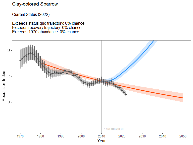
Below, we illustrate a population projection for Clay-colored Sparrow. For illustrative purposes, we imagine that in 2010 a goal was set to increase population growth rate by +0.5% per year, until a growth rate of +3% per year was achieved. We plot the resulting “recovery projection”, and track progress towards that goal by comparing the empirical population indices (from 2011 to 2022) against the projection.

The code below accomplishes this projection, using a custom R function called projection_function:

CCSP_projection <- projection_function(CCSP_results,
                                       
                                       # Years for calculating baseline index for 'full recovery' (average across these years)
                                       baseline_years = c(1980,1981,1982,1983,1984),    
                                       
                                       # How far back to calculate "current" trend over)
                                       length_current_trend = 30, # 30 year trend
                                       
                                       # Year in which goals were set
                                       year_goals_are_set = 2010,
                                       
                                       # Percent change per year once population reaches its target growth rate
                                       target_trend = 3,    
                                       
                                       # Goal is to increase growth rate by 0.5% per year, until target it reached
                                       annual_growth_rate_improvement = 0.5,
                                       
                                       # Final year of projection
                                       end_of_projection = 2050
)

The blue curve represents the recovery scenario.

The red curve represents a population that continues to decline at the mean long-term rate observed for the population.

The gray curve is the trajectory the population has actually taken.

All of the data and projection curves could be expressed relative to a historical baseline population index. In this case, we use the mean population index from 1980-1984 as a baseline abundance which would represent “full recovery” of the species. Nothing has changed in terms of the model inputs, assumptions, or outputs; this is just a different way of graphically visualizing the projections.

The plot below illustrates this alternative way of visualizing the projections:

This framework illustrates several key messages:

Currently, the national population of Clay-colored Sparrow is almost certainly below the recovery target that was set for it as of 2010 (>99.9% chance). Moreover, the current population estimate is currently even lower than if the population had continued to decline at its long-term rate. This implies that since 2010, the population has declined more rapidly than its long-term mean rate of change.
If recovery targets are met, in the year 2050 the population would be at 221.2% of its baseline abundance (95% CRI = 198.9 to 244%).
If the recovery target is met, we expect the population to achieve “full recovery” in the year 2024 (95% CRI = 2020 to 2027).

Application to all species

We applied the framework to _____ species that are estimated to have experienced long-term population declines and are considered to be well-monitored by the Breeding Bird Survey. For each species, we set population goals starting in 2022 (the most recent year of BBS estimates).

This involved:

Fitting Bayesian hierarchical models for each species, to estimate population trajectories and historical trends
Conducting projections of population recovery, assuming population growth rates would be increased by 0.5% per year until a target growth rate of +3% per year was achieved (after which, the projection continued growing at a rate of +3% per year)
Reporting the population status in 2050 (i.e., under the hypothetical scenario where the population grew according to the projection)
Reporting the year in which ‘full recovery’ would be achieved (i.e., under the hypothetical scenario where the population grew according to the projection)

Code to accomplish this is shown below:

target_species <- read_xlsx("data/species with long term declines (12dec2023).xlsx")

for (species_name in target_species$Species){
  
  # 4 letter species abbreviation code
  sp_code <- subset(ac, English_Name == species_name)$Species_ID
  
  # Directory where fitted model will be stored 
  filename <- paste0("fitted_models/",sp_code,".RDS")
  
  # Fit model for this species, save resulting indices
  if (!file.exists(filename)){
    
    # Stratify data
    s <- stratify(by = "bbs_usgs", species = species_name)
    
    p <- tryCatch(expr = {prepare_data(s)},
                  error = function(e){NULL})
    
    # Fit model & generate indices
    if (is.null(p)) next
    p <- prepare_data(s)
    md <- prepare_model(p, model = "gamye")
    m <- run_model(md, save_model = FALSE)
    i <- generate_indices(model_output = m, regions = "country")
    
    # National indices
    samps <- i$samples$country_Canada
    
    # Save results
    sp_results <- list(samps = samps)
    saveRDS(sp_results, file = filename)
    
    # Generate projections
    sp_projection <- projection_function(
      
      sp_results,
      
      # Years for calculating baseline index for 'full recovery' (average across these years)
      baseline_years = c(1980,1981,1982,1983,1984),    
      
      # How far back to calculate "current" trend over)
      length_current_trend = 30, # 30 year trend
      
      # Year in which goals were set
      year_goals_are_set = 2022,
      
      # Percent change per year once population reaches its target growth rate
      target_trend = 3,    
      
      # Goal is to increase growth rate by 0.5% per year, until target it reached
      annual_growth_rate_improvement = 0.5,
      
      # Final year of projection
      end_of_projection = 2100
    )
  }
}

Results summaries

A full set of results were produced by the script projection.R.

Tabular summaries of population projection results are stored in /summary_tables/projection_table.csv.

Plots of projections for each species are stored in /summary_figures/.

Extensions

This framework can be applied to species that are monitored by other programs than the BBS (e.g., for species better-monitored by the Christmas Bird Count, migration monitoring, targeted surveys, etc). To fully propagate uncertainty in projections, the framework requires a time series of population estimates with uncertainty represented by a collection of samples from a joint Bayesian posterior. For species that are not modeled using Bayesian methods, bootstrapping can be used to construct a collection of population time series (which represent uncertainty in the empirical estimates of how populations have changed over time).

Citations

R Core Team (2021). R: A language and environment for statistical computing. R Foundation for Statistical Computing, Vienna, Austria.

AdamCSmithCWS/Interim_Goals_Framework