My-CarND-Advanced-Lane-Lines-Submission: A Jupyter Notebook repository from Alexspayne

I just used this file so that I could use Jupyter's markdown preview.

Advanced Lane Finding Project

The goals / steps of this project are the following:

Compute the camera calibration matrix and distortion coefficients given a set of chessboard images.
Apply a distortion correction to raw images.
Use color transforms, gradients, etc., to create a thresholded binary image.
Apply a perspective transform to rectify binary image ("birds-eye view").
Detect lane pixels and fit to find the lane boundary.
Determine the curvature of the lane and vehicle position with respect to center.
Warp the detected lane boundaries back onto the original image.
Output visual display of the lane boundaries and numerical estimation of lane curvature and vehicle position.

Rubric Points

Here I will consider the rubric points individually and describe how I addressed each point in my implementation.

Writeup / README

1. Provide a Writeup / README that includes all the rubric points and how you addressed each one. You can submit your writeup as markdown or pdf. Here is a template writeup for this project you can use as a guide and a starting point.

You're reading it! Most of the code is in the advanced_lane_finding.ipynb.

Camera Calibration

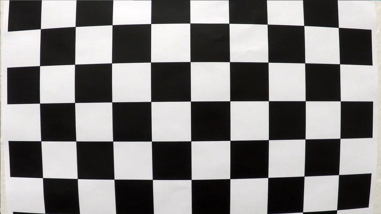
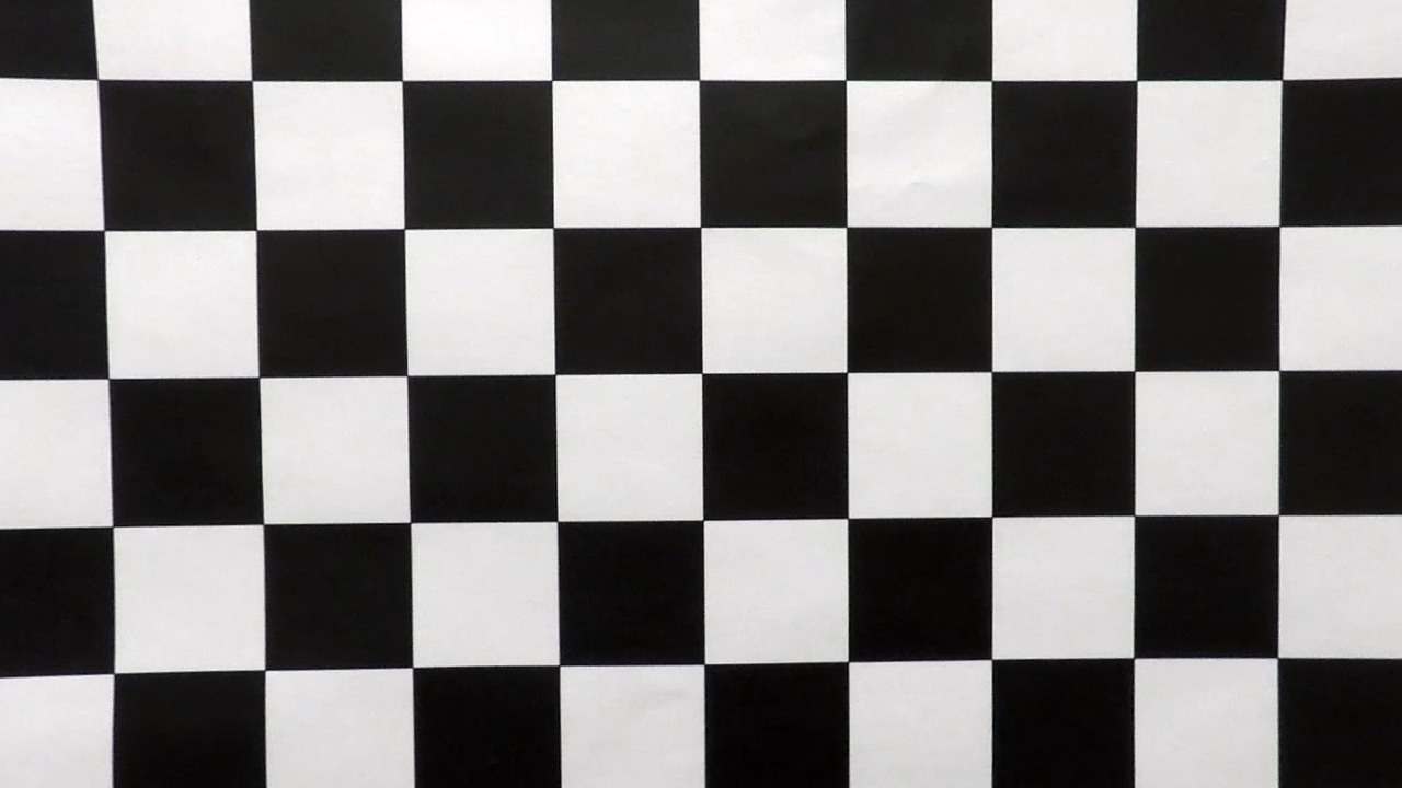
1. Briefly state how you computed the camera matrix and distortion coefficients. Provide an example of a distortion corrected calibration image.

The code for this step is contained in the first code cell of the Jupyter notebook "advanced_lane_finding.ipynb"

I start by preparing "object points", which will be the (x, y, z) coordinates of the chessboard corners in the world. Here I am assuming the chessboard is fixed on the (x, y) plane at z=0, such that the object points are the same for each calibration image. Thus, objp is just a replicated array of coordinates, and objpoints will be appended with a copy of it every time I successfully detect all chessboard corners in a test image. imgpoints will be appended with the (x, y) pixel position of each of the corners in the image plane with each successful chessboard detection.

I then used the output objpoints and imgpoints to compute the camera calibration and distortion coefficients using the cv2.calibrateCamera() function. I applied this distortion correction to the test image using the cv2.undistort() function and obtained this result:

Original Image

Undistorted Image

Pipeline (single images)

1. Provide an example of a distortion-corrected image.

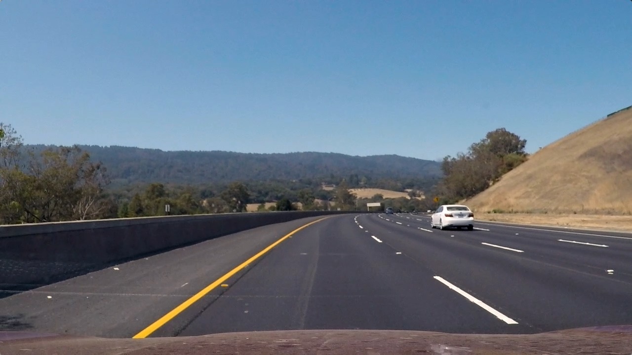
To demonstrate this step, I will describe how I apply the distortion correction to one of the test images like this one: [image2]: ./output_images/Undistorted_Test_Image.jpg "Road Transformed" [original2]: ./output_images/Original_Test_Image.jpg "Original Image"

Original Image

![alt text][original2]

Undistorted Image

![alt text][image2]

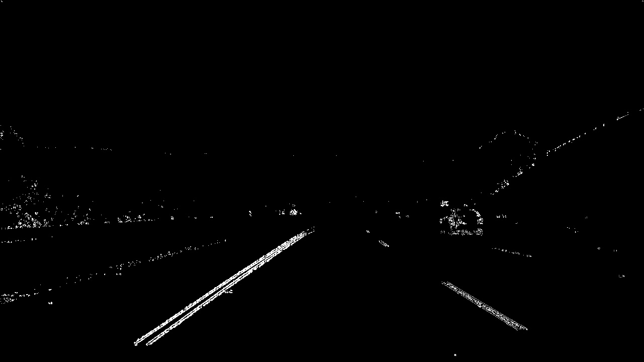
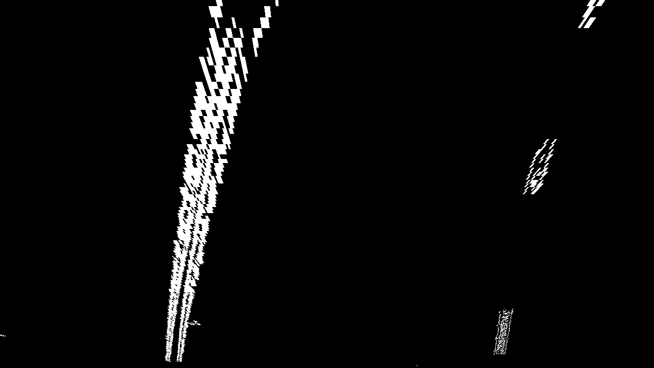
2. Describe how (and identify where in your code) you used color transforms, gradients or other methods to create a thresholded binary image. Provide an example of a binary image result.

The functions I used for thresholding are found in binarythresholding.py.
The pipeline is shown in the first cell of the Applying thereshold to produce a binary image section of the Jupyter notebook advanced_lane_finding.ipynb

I derived reasonably good threshold values by using a tool I wrote in the last code cell of Notes/Combination.ipynb

Here's a picture of that: [tool]: ./output_images/matplotlibSlider.png "Finding Parameters" ![alt text][tool]

Here are the steps for this part of the pipeline:

Extract the saturation channel.
Apply a sobel threshold in both the x and y direction, as well as a magnitute gradient.
Take the intersect of points from each of the three thresholds to make the final binary.

Here's an example of my output for this step.

Original Image

Binary Image

3. Describe how (and identify where in your code) you performed a perspective transform and provide an example of a transformed image.

The code for my perspective transform includes a function called warper(), which appears in the code cell directly under the heading Apply a perspective transform to rectify binary image ("birds-eye view"). in the Jupyter notebook). The warper() function takes as inputs an image (img), as well as source (src) and destination (dst) points. I chose the hardcode the source and destination points in the following manner:

src = np.float32(
    [[(img_size[0] / 2) - 55, img_size[1] / 2 + 100],
    [((img_size[0] / 6) - 10), img_size[1]],
    [(img_size[0] * 5 / 6) + 60, img_size[1]],
    [(img_size[0] / 2 + 55), img_size[1] / 2 + 100]])
dst = np.float32(
    [[(img_size[0] / 4), 0],
    [(img_size[0] / 4), img_size[1]],
    [(img_size[0] * 3 / 4), img_size[1]],
    [(img_size[0] * 3 / 4), 0]])

This resulted in the following source and destination points:

Source	Destination
585, 460	320, 0
203.3, 720	320, 720
126.6, 720	960, 720
695, 460	960, 0

I verified that my perspective transform was working as expected by drawing the src and dst points onto a test image and its warped counterpart to verify that the lines appear parallel in the warped image.

Original Image

Warped Image

4. Describe how (and identify where in your code) you identified lane-line pixels and fit their positions with a polynomial?

I used the sliding window method implementation provided by Udacity (code in the Jupyter notebook under the Detect lane pixels and fit to find the lane boundary. heading.)

The sliding window method follows these steps:

Generate a histogram against the bottom half of the binary image
Use the peaks to determine the location of the lane lines at the bottom of the image
Find the rectangle with the most activated pixels in each rectangular column of the image.
Add that rectangle to an array.
Fit a second order polynomial to the pixel positions derived from the array of rectangles.
Repeat steps 3-5 for each new frame using the base search location from the first frame.

Here is the result of the method applied to the binary image: The green boxes represent the rectangles bounding the lane line at each column. The yellow line represents the poloynomial function that was fit to each lane line. [image5]: ./output_images/polyfit_result.png "Fit Visual" ![alt text][image5]

5. Describe how (and identify where in your code) you calculated the radius of curvature of the lane and the position of the vehicle with respect to center.

I did this in the Jupyter notebook under the heading: "Determine the curvature of the lane and vehicle position with respect to center."

The steps I took to find the radius of curvature the same as Udacity's approach in the lesson.

Convert the distance measurements from pixels to meters.
Fit a polynomial to the lane pixels using meters instead of just pixels.
I applied the radii using the formula for the radius of the curvature.
Often the radius of the curvature was way off for the dashed lane lines. To combat this, I gave preference to the radius from the line that was closest to the trend when reporting the radius.

To find the position of the vehicle from the center lane, used the same method as described in the Q&A.

For each y value, find the midpoint between the left and right lane by taking the average.
Compare this midpoint to the center of the image to get the difference.
Convert this pixel difference to meters.
Determine which side of the centerline the vehicle is on by checking the sign of the difference.

See the image in step 6 for an example.

6. Provide an example image of your result plotted back down onto the road such that the lane area is identified clearly.

This step is carried out under the heading Warp the detected lane boundaries back onto the original image.

Here is an example of my result on a test image: [plotted]: ./output_images/vehicle_heading.jpg "Output"

![alt text][plotted]

Pipeline (video)

1. Provide a link to your final video output. Your pipeline should perform reasonably well on the entire project video (wobbly lines are ok but no catastrophic failures that would cause the car to drive off the road!).

Here's a link to my video result

Discussion

1. Briefly discuss any problems / issues you faced in your implementation of this project. Where will your pipeline likely fail? What could you do to make it more robust?

The application got slightly confused in two cases:

Being passed by a car with bright wheels.
Passing under a shadow.

To solve these problems, I could try the following things:

I could add averaging to prevent it from jumping to detecting wheels.
I could limit the search for the lane lines to a small window around the last found lane lines.
I could modify the field of view so that the model can't see very far into adjacent lanes.

Some other potential issues:

Heavy traffic
The vehicle changing lanes
Weather

Alexspayne/My-CarND-Advanced-Lane-Lines-Submission

Rubric Points

Here I will consider the rubric points individually and describe how I addressed each point in my implementation.

Writeup / README

1. Provide a Writeup / README that includes all the rubric points and how you addressed each one. You can submit your writeup as markdown or pdf. Here is a template writeup for this project you can use as a guide and a starting point.

Camera Calibration

1. Briefly state how you computed the camera matrix and distortion coefficients. Provide an example of a distortion corrected calibration image.

Original Image

Undistorted Image

Pipeline (single images)

1. Provide an example of a distortion-corrected image.

Original Image

Undistorted Image

2. Describe how (and identify where in your code) you used color transforms, gradients or other methods to create a thresholded binary image. Provide an example of a binary image result.

Original Image

Binary Image

3. Describe how (and identify where in your code) you performed a perspective transform and provide an example of a transformed image.

Original Image

Warped Image

4. Describe how (and identify where in your code) you identified lane-line pixels and fit their positions with a polynomial?

5. Describe how (and identify where in your code) you calculated the radius of curvature of the lane and the position of the vehicle with respect to center.

6. Provide an example image of your result plotted back down onto the road such that the lane area is identified clearly.

Pipeline (video)

1. Provide a link to your final video output. Your pipeline should perform reasonably well on the entire project video (wobbly lines are ok but no catastrophic failures that would cause the car to drive off the road!).

Discussion

1. Briefly discuss any problems / issues you faced in your implementation of this project. Where will your pipeline likely fail? What could you do to make it more robust?