(I)nferred Drug (S)ensitivity (O)perating on the integration of (S)ingle-(C)ell (E)xpression and (L)1000 (E)xpression (S)ignatures
Explore the docs »
Report Bug
·
Request Feature
Table of Contents
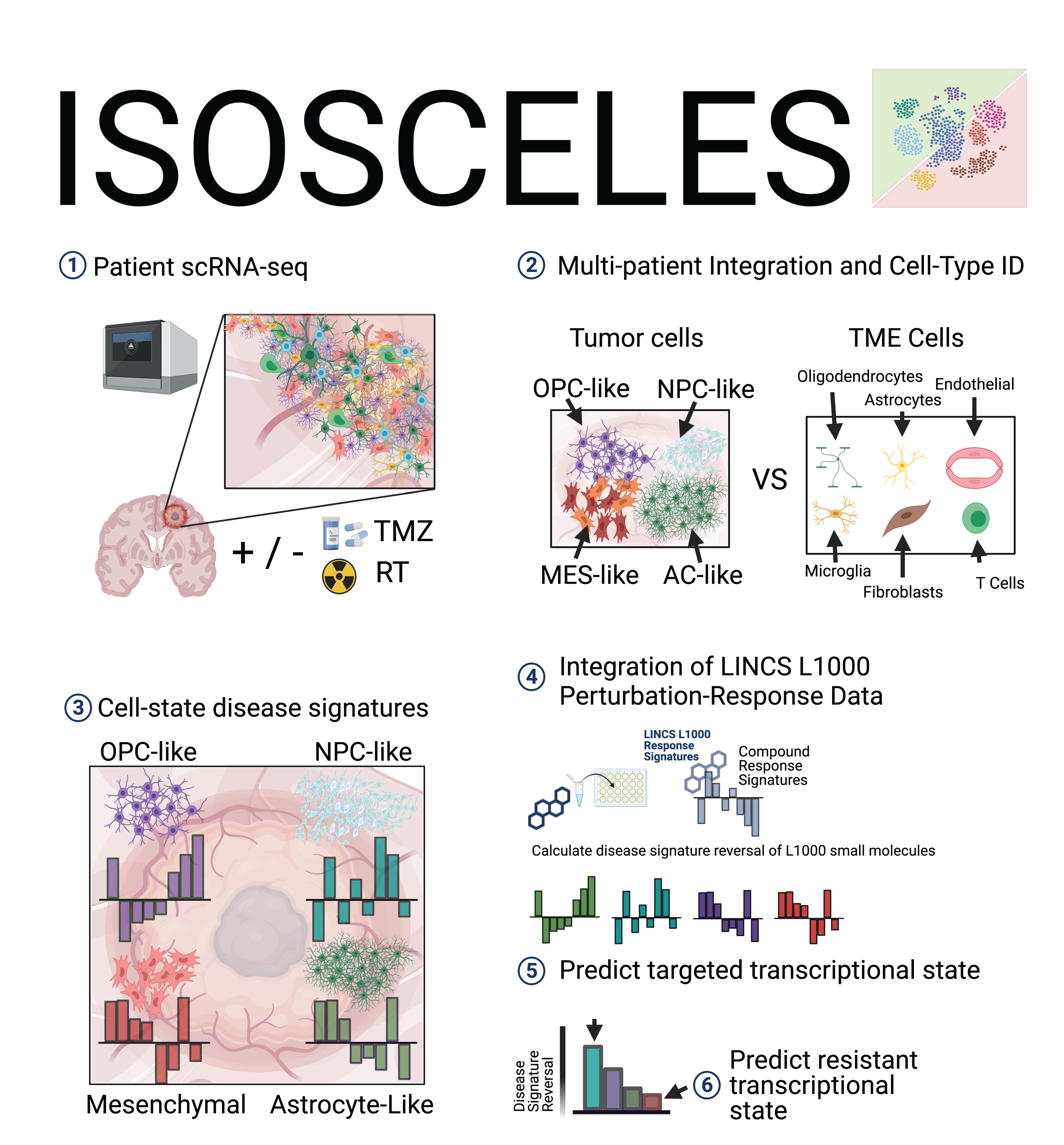
ISOSCELES operates through the integration of drug-response transcriptional consensus signatures (TCSs) derived from the LINCS L1000 dataset with multi-subject single-cell RNA sequencing data, and facilitates analysis of drug and cell connectivity as a function of expression discordance from multiple perspectives.
You can find ISOSCELES on shinyapps.io here! »
Due to the inherent large size of scRNAseq datasets, we highly recommend installing the ISOSCELES R package to run the application locally.
The ISOSCELES R package for R > 4.3.0 can be installed with devtools.
Installation of devtools in R:
# Install devtools from CRAN
install.packages("devtools")

# Or the development version from GitHub:
# install.packages("devtools")
devtools::install_github("r-lib/devtools")
ISOSCELES requires the following additional R packages:
library(shiny)
library(Seurat)
library(ggplot2)
library(tibble)
library(cowplot)
library(viridis)
library(dplyr)
library(ggsci)
library(ggrepel)
library(tidyverse)
library(plotly)
library(htmlwidgets)
library(reshape2)
library(Hmisc)
library(corrplot)
library(pheatmap)
library(grid)
library(MAST)
library(shinydashboard)
library(shinythemes)
library(scales)
library(ggforce)
library(EnhancedVolcano)
library(DT)
Some of these dependencies will need to be installed via Bioconductor.
Installation of BiocManager:
if (!require("BiocManager", quietly = TRUE))
    install.packages("BiocManager")
BiocManager::install(version = "3.17")
and to install core bioconductor packages:
BiocManager::install()
Using devtools, the ISOSCELES R package can be installed from the source file. With all dependencies satisfied, installation should take less than 5 minutes.
Download the ISOSCELES source file here! »
devtools::install_local("pathToYourSourceFile/ISOSCELES_0.0.0.9000.tar.gz")
Follow this brief tutorial below to familiarize yourself with the application.
Once installed, launching ISOSCELES is as easy as the following:
library(ISOSCELES) # load the ISOSCELES library including necessary drug signature data
ISOSCELES::runISOSCELES() # launch the ISOSCELES shiny GUI
ISOSCELES takes scRNAseq input in the form of a Seurat object saved as an RDS file.
Simply choose your file to upload and allow the app to load the Seurat object into the processing environment. Once it is fully loaded, you will see a prompt for the successful upload and to proceed to the pre-processing step.
You can download a small example RDS file of a seurat object subsetted from our data presented within our manuscript here:
Download a subsampled version of our processed Seurat object available on GEO! »
Please note - this sub-sampled object only contains 500 out of greater than 100,000 cells analyzed within our manuscript to facilitate an accessible usage example. Findings from this subsample will not be representative of those resulting from analysis of the full scRNAseq analyzed within the manuscript. Subsampling was performed as follows:
library(Seurat)
set.seed(1)

obj_toSub <- readRDS(file = "seuratObj.RDS")
downsampled.obj <- obj_toSub[, sample(colnames(obj_toSub), size = 500, replace=F)]
saveRDS(downsampled.obj, file = "downsampled_seuratObj.RDS")
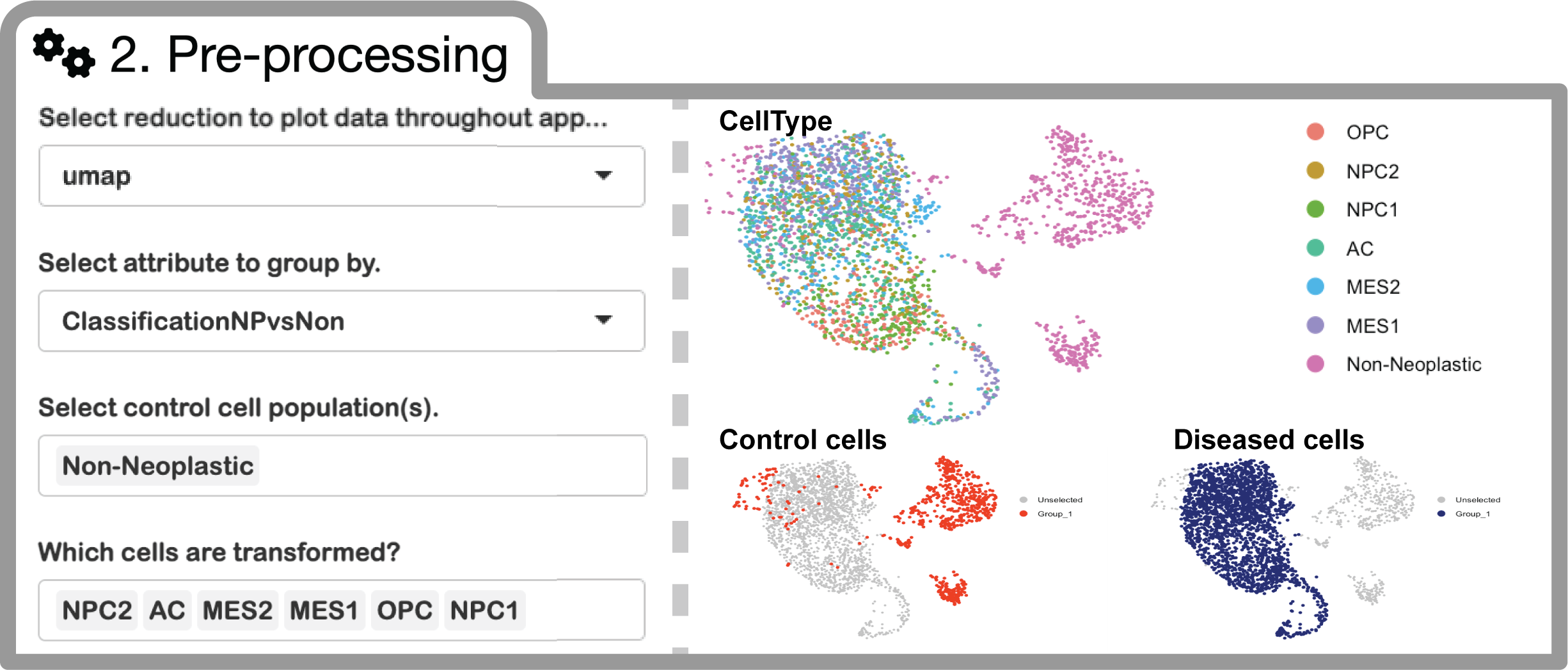
Analysis with ISOSCELES requires identification of tumor cell subpopulations, and non-tumor TME cell populations (control cell populations) using annotations within the metadata of your uploaded Seurat object. (i.e. obj@meta.data$cellType). Make sure that your annotations of interest are saved within your RDS file.
Here, you may select the dimensionality reduction to use to visualize your data throughout the app (i.e. UMAP, PCA, any custom reduction, etc.).
You will also select the relevant metadata column to group your cells by. Once selected, you will be able to select the individual identities within those annotations identifying transformed tumor cells (for GBM, we chose to group by GBM cell transcriptional state (Neftel et al., 2019) and your control populations (non-tumor cell types). Your selections will be visualized by coloring selected cells based on their grouping as control cells or diseased cells.
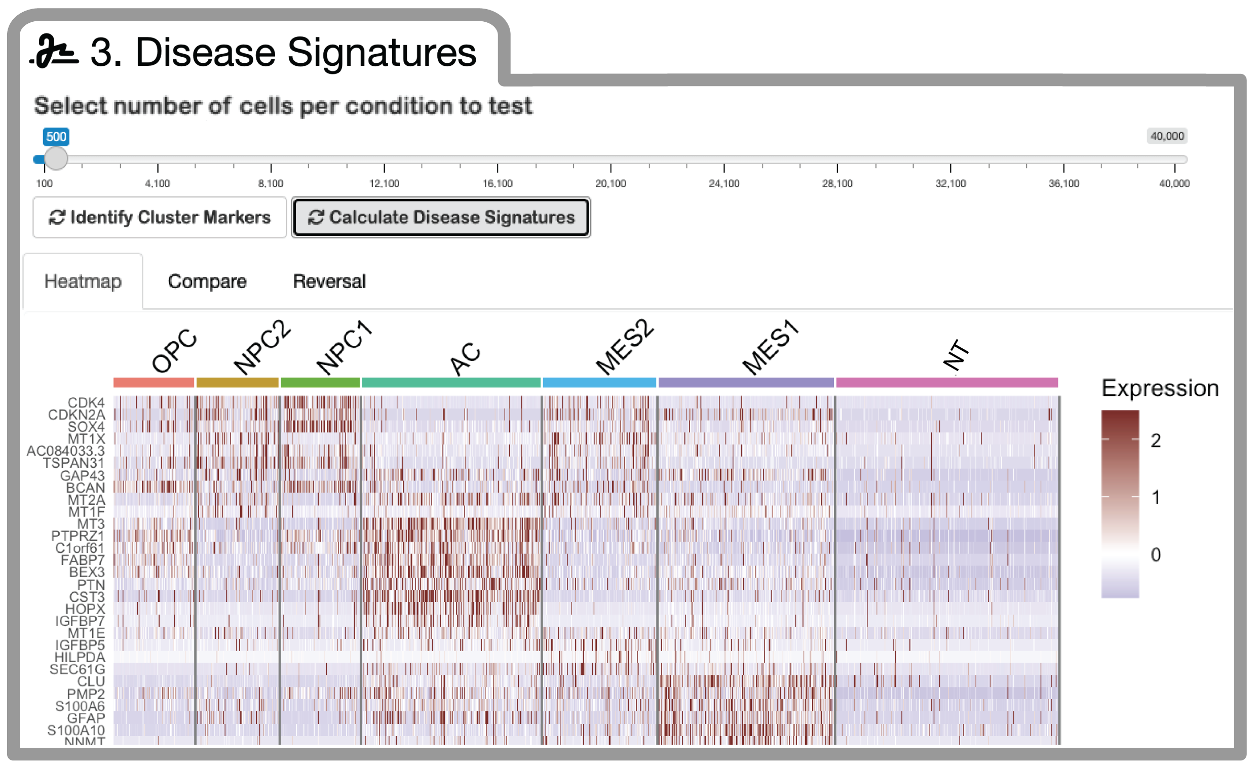
Based on your test (transformed / diseased) and control cell populations selected during pre-processing, you can now generate cell-state (or type) specific disease signatures.
A slider allows you to sub-sample cells within each identity in order to speed up processing.
Once completed, a heatmap will be generated to visualize the expression of top disease signature genes across all cells in your dataset.
You can now navigate to the 'Compare' and 'Reversal' tabs to analyze and visualize disease signature correlations across tumor cell identities, and to score small molecules from the L1000 dataset for the reversal of these respective disease signatures. Disease signature and reversal score output can be downloaded as .csv files.
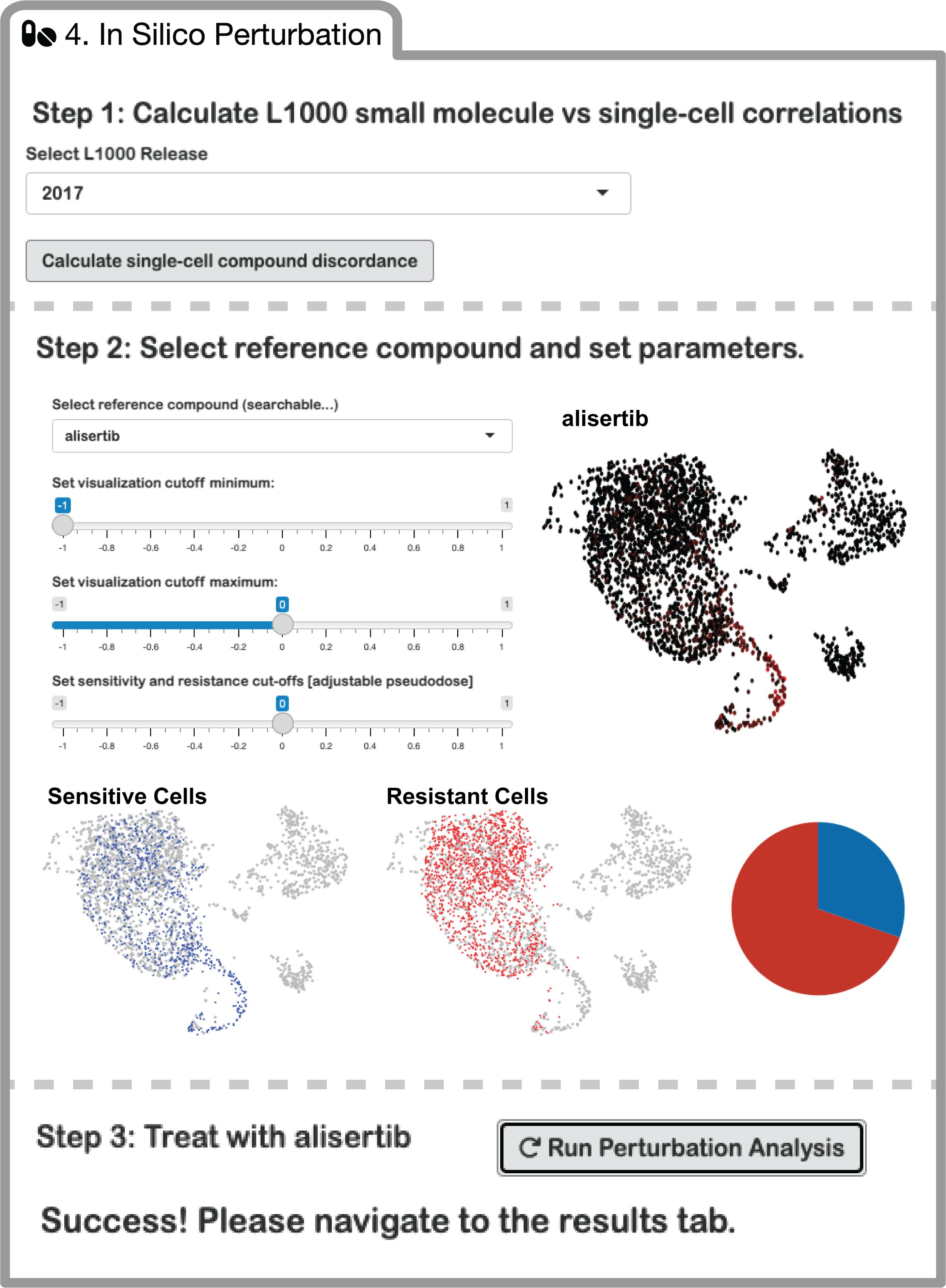
ISOSCELES' Drug-Cell connectivity analysis scores cells for their concordance or discordance with small molecule perturbation response signatures, to identify resistant and sensitive tumor cells, respectively.
Simply select the L1000 release date (currently 2017 is the only working option, new releases will be added to the application soon), and calculate Drug-Cell expression correlations. These results are downloadable, and can be uploaded back to the application so that this calculation does not need to be run repetitively.
Download a pre-calculated Drug-Cell Connectivity Matrix for the subsampled example dataset here! »
runtime: Initial scoring of Drug-Cell connectivity is the most computationally expensive portion of this software. On our example dataset of only a few hundred cells, this step should run in less than 20 minutes on a 'normal' desktop computer. Upload of connectivity score matrix functionality is provided to cut down on compute time for future analyses.
Once the Drug-Cell connectivity matrix is generated, the window below will populate, and you may select a compound of interest to perform an in silico perturbation experiment on your scRNAseq data with. Once selected, a threshold for sensitivity and resistance (i.e. pseudodose) can be selected. Cells deemed sensitive or resistant will be visualized, as well as the proportions of cells within each grouping. Clicking the run button will prepare the environment for step 5, visualization of results.
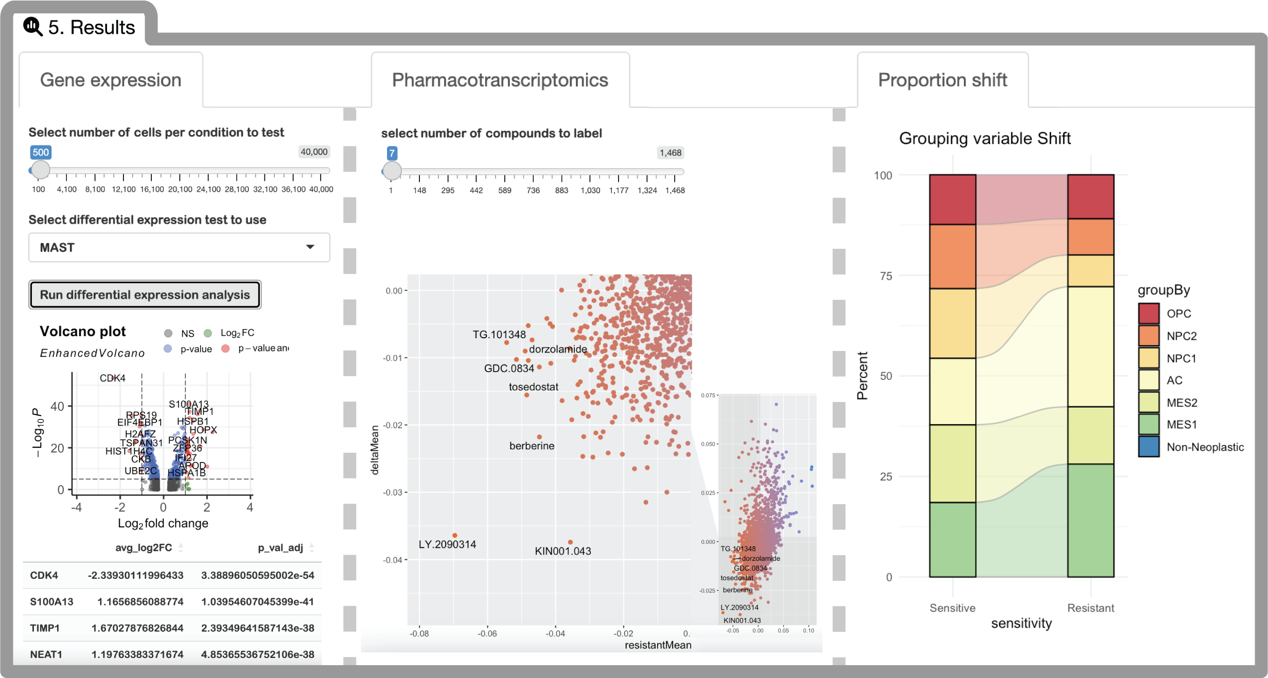
Under the results tab, you will be able to analyze differences between ISOSCELES predicted sensitive and resistant populations, including gene expression, proportions of discrete cell identities, as well as pharmacotranscriptomic properties across the entire L1000 dataset. The interpretation of these findings is explained in-depth within our manuscript.
Contributions are what make the open source community such an amazing place to learn, inspire, and create. Any contributions you make are greatly appreciated.
If you have a suggestion that would make this better, please fork the repo and create a pull request. You can also simply open an issue with the tag "enhancement".
- Fork the Project
- Create your Feature Branch (
git checkout -b feature/AmazingFeature) - Commit your Changes (
git commit -m 'Add some AmazingFeature') - Push to the Branch (
git push origin feature/AmazingFeature) - Open a Pull Request
Not currently distributed under any license. Public for manuscript review.
Robert K. Suter, PhD - @biovibin - rks82@georgetown.edu
Nagi G. Ayad, PhD - @nagi_ayad - na853@georgetown.edu
Project Link: https://github.com/AyadLab/ISOSCELES


