GeneralizedCoarseGraining

Generalized Coarse Graining (GCG) enables the recursive coarse graining of discrete energy landscapes into gradient basins, funnels, super funnels, ..., using a gradient-neighbor-based aggregation directive.

`gcgBarriers.pl`

The Perl5 script gcgBarriers.pl computes the gradient-based coarse graining of a given energy landscape encoding as produced by the barriers tool when enabling full rate computation activated by its --rates argument.

Usage: perl gcgBarriers.pl <barriersOutput> <barriersRates>

RNA example

The following call set exemplifies the usage of gcgBarriers.pl for the RNA secondary structure energy landscape of riboswitch f07-a using the Vienna RNA package. Note, the calls are only viable for very short sequences since the whole accessible structure space / energy landscape is considered.

# define RNA sequence of interest
RNA=GACCGGAAGGUCCGCCUUCC

# enumerate (and sort) all secondary structures (first by energy using structure string for tie breaking)
echo $RNA | RNAsubopt --deltaEnergy=99999 | sort -k 2,2n -k 1,1dr -S 2G | zip $RNA.RNAsubopt.zip -;

# run barriers to compute coarse graining level 1
unzip -p $RNA.RNAsubopt.zip | barriers --rates -G RNA -M noShift --bsize --max=999999 --minh=0 > $RNA.barriers.out;
# store rate matrix generated by barriers
mv rates.out $RNA.barriers.rates;
# cleanup obsolete barriers files
rm -f rates.bin tree.ps treeR.ps;

# compute generalized coarse grainings
perl gcgBarriers.pl $RNA.barriers.out $RNA.barriers.rates

The calls produce the output

level number
level states
0 2993
1 39
2 7
3 1

which states the number of macro-states on each coarse graining level. Furthermore, the following files for each coarse graining level (LVL) > 1 are generated:

*.LVL.gradient : appends an additional column to the barriers output file of the compressed level (LVL-1), which contains the gradient assignment for each local minimum
*.LVL.barriers : a dummy barriers output file for the current level
*.LVL.rates : the rates matrix for the current level

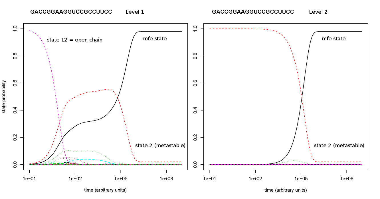
Given this data, you can plot the probability time series for the macro-states using treekin.

# define variables for the following shell function
FILE="undef"; # base file name without extension (.barriers .rates)
OCID=0; # funnel of open chain state to be taken from according barriers output file
STEPS=1000000000; # maximal time (step) to compute
# shell function (tested in bash) to compute one plot via treekin 
function runTreekin {
 # ensure file naming for treekin call
 ln -s $FILE.rates rates.out;
 # output file prefix 
 OUTFILE=$FILE.treekin.m$OCID
 # call treekin
 treekin -m I --p0 $OCID=1  --t8=$STEPS < $FILE.barriers > $OUTFILE.out; 
 # cleanup temporary files
 rm -f rates.out;
 # generate output figure in pdf format using R
 R --vanilla --silent -e "k <- read.table(\"$OUTFILE.out\", header=F, sep=\"\");pdf(\"$OUTFILE.pdf\");matplot(k[,1], k[,2:ncol(k)], main=\"$OUTFILE\", xlab=\"time (arbitrary units)\", ylab=\"state probability\", ylim=c(0,1), log=\"x\", type=\"l\");dev.off(); q();"
}

# define RNA sequence of interest
# e.g. riboswitch from https://doi.org/10.1002/bip.20761 Fig.7(left)
RNA=GACCGGAAGGUCCGCCUUCC

# level 1 plot
ln -s -f $RNA.barriers.out $RNA.barriers.out.1.barriers
ln -s -f $RNA.barriers.rates $RNA.barriers.out.1.rates
FILE=$RNA.barriers.out.1
OCID=12 # open chain state
runTreekin

# level 2 plot
FILE=$RNA.barriers.out.2
OCID=2 # gradient neighbor of open chain state from level 1
runTreekin

which will generate the following figures

Used program versions for the example output: ViennaRNA-2.4.4, barriers-1.6.0, treekin-0.3.1

BackofenLab/GeneralizedCoarseGraining

GeneralizedCoarseGraining

gcgBarriers.pl

RNA example

`gcgBarriers.pl`