Original Udacity Project Repo CarND-Advanced-Lane-Lines
The goals / steps of this project are the following:
- Compute the camera calibration matrix and distortion coefficients given a set of chessboard images.
- Apply a distortion correction to raw images.
- Use color transforms, gradients, etc., to create a thresholded binary image.
- Apply a perspective transform to rectify binary image ("birds-eye view").
- Detect lane pixels and fit to find the lane boundary.
- Determine the curvature of the lane and vehicle position with respect to center.
- Warp the detected lane boundaries back onto the original image.
- Output visual display of the lane boundaries and numerical estimation of lane curvature and vehicle position.
The code is in Python notebook located in "parameter_tuning.ipynb" under Camera Calibration section. You can also view this in markdown format here parameter_tuning
Since I am calibrating the camera using a 9 by 6 chessboard on a flat surface, I have created a variable called objpoints that will hold x and y coordination of this 9 by 6 matrix with z = 0, i.e. (0,0,0) ,(1,0,0),(0,1,0)...and so on. This objpoints would be the same for all calibration image using this chessboard.
Then I used cv2.findChessboardCorners to find all x and y coordinates of those chessboard corners in each calibration images that took in different angles.

By using a "for loop" to scan through all the calibration images, I appended all image points found by cv2.findChessboardCorners into imgpoints and its matching of objpoints.
Next, I used those points and executed cv2.calibratCamera to obtained mtx,dist that can be used for cv2.undistort. Following images are the example of the undistorted images

To simplify later video processing code, I created a .py script for camera calibration so I just call this function. The py script is at "frame_process.py"
In that script, I created a global variable cali that will hold mtx,dist. In def undistort_img(img), I will make sure this calibration only done once when this scripted is called to save runtime.
To demonstrate this step, I will describe how I apply the distortion correction to one of the test images like this one:

In the "parameter_tuning.ipynb", I printed out all the undistorted images for reference and they are also located at "./undistort_test_images"
I have run rgb, hsv, and hls to every test image to see which color filter would work the best among all the images. In the end, I concluded S and L in HLS, combined with R in RGB would be the channels I would use to do the color filtering.
I also experimented the magnitude, directional and absolute gradients to find out the proper threshold values. I tested out the runtime of those algorithm, and decided to implement a flag called overdrive to choose to run only absolute gradient or all gradient combined. The runtime difference is around 1 s per frame and this will save a lot of time when processing a video.
The logic I used to combine those gradients is
if overdrive:
        mag_binary = mag_threshold(gray,sobel_kernel=ksize,thresh= mag_thresh)
        dir_binary = dir_threshold(gray, sobel_kernel=ksize, thresh=dir_thresh)
        combined[((gradx == 1) & (grady == 1)) | ((mag_binary == 1) & (dir_binary == 1))] = 1
    else:
        combined[(gradx == 1) & (grady == 1)] = 1
Following thresholds are applied:
| Item | Threshold Range |
|---|---|
| H in HSL | (23, 100) |
| S in HSL | (170, 255) |
| R in RGB | (220, 255) |
| abs gradient | (50, 200) |
| mag gradient | (60, 150) |
| dir gradient | (0.7,1.3) |
After experiment with all the threshold values, I created a function called image_process to combining all the process and output an binary image. When overdrive flag is set, one of colored output (R:R in RGB; G:Color filter result;B:Combined Gradient Result) is like:

For the perspective transform, I have defined two functions: mask_image() and perspective_transform().
mask_image is used to define the source and destination coordinates for perspective transform. The source four points are defined by input of mask_top_width (the top width of the trapezoid), x_offset (the distance of the bottom x coordinate of the trapezoid to the edge of the image in X direction),y_offset (the distance of the bottom y coordinate of the trapezoid to the edge of the image in Y direction) . Calculation shown as below:
    imshape=img.shape
    # Calculate mask height
    img_y_mid = imshape[0]*0.5
    mask_height = int(img_y_mid*1.25)
    img_x_mid = int(imshape[1]*0.5)
    top_left = [img_x_mid - mask_top_width*0.5 , mask_height]
    top_right = [img_x_mid + mask_top_width*0.5 , mask_height]
    bottom_left = [x_offset,imshape[0]-y_offset]
    bottom_right = [imshape[1]-x_offset,imshape[0]-y_offset]
For the Destination coordinates, I simply defined as
# 25 is hardcoded to move the lane line to the bottom of the image
    dst = np.float32([[dst_offset, imshape[0]-y_offset+25], [dst_offset, y_offset],
                                     [imshape[1]-dst_offset, y_offset],
                                     [imshape[1]-dst_offset, imshape[0]-y_offset+25]])
I verified that my perspective transform was working as expected by drawing the src and dst points onto a test image and its warped counterpart to verify that the lines appear parallel in the warped image.

In the "frame_process.py", I combined all the process in binary_wrop_img(). This function will call for mask_image() to have src and dst and call image_process() to get the binary image and then wrap the image using perspective_transform().
From now on, all the code has been saved to a different notebook to be more neat.
The notebook file is called Advance_pipeline.ipynb
To identify the lane-line pixels, I decided to have a logic process one line at a time. Instead of running two lines in one function, I am able to run only one line if the previous result is bad while the other line has a high confident result.
if the line is hard to find or previous result is not so confident, I run find_lane_pixels() that uses a more time consuming sliding windows logic.
If the previous result is accurate, I will run search_around_poly to search an area around last poly fit result to save runtime.
If there are a number of failed to detect lines, I will flag overdrive to True and run a more complex and time consuming image_process() to obtain a more accurate input before the pixel finding logic.
Fit polynomial code and curvature calculation are in fit_one_line().
curvature calculation is in fit_one_line().
To convert pixels to meters, I used following values:
    ym_per_pix = 3 / 80
    xm_per_pix = 3.7 / 570
And the radius of curvature is curve_rad = (1 + (2 * fit_cr[0] * y_eval * ym_per_pix + fit_cr[1]) ** 2) ** 1.5 / np.absolute(2 * fit_cr[0])
I implemented this step in my code in Advance_pipline.ipynb in the function video_lane_detection(). Here is an example of my result on a test image:

1. Provide a link to your final video output. Your pipeline should perform reasonably well on the entire project video (wobbly lines are ok but no catastrophic failures that would cause the car to drive off the road!).
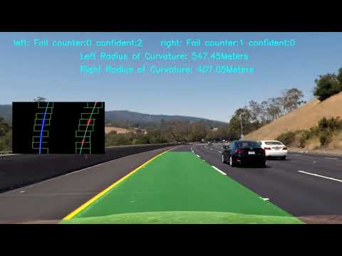
As you can see in the final video, the lane finding logic switching between sliding windows and search around poly to save run time. Also, around 20s in the video, you will see the lane detection fail to detect lanes but the mask lane would remain proximately in the same area due to the average and slope check logic.
1. Briefly discuss any problems / issues you faced in your implementation of this project. Where will your pipeline likely fail? What could you do to make it more robust?
My Pipeline uses a counting up confident level to determine how the current iteration is compare to the previous result. This works on a stable and continuous good input image that yield consistent binary wrap images. Additionally, the logic to judge the confident uses relative percentage of previous result, which would contribute more error if the algorithm continuously failed to detect.
Therefore, if the fail count is greater than 30 times, the result stored in the Line class would not be accurate enough for the confident check to work properly. That's why when the car is turning and the algorithm is keep failing to detect, the left line detection was not able to quickly adapt to the change.
To improve this, if I have more time to work on this, I would use if function directly to throw away some very far off results based on the line to the center distance and slope change. I would also create a logic that can detect the car is turning, increase the threshold on confident checks to run smoothly around the corner.
I also notice my pipeline would go nuts on challenge video due to no correct line pixels found in sliding window logic. I would add logic to handle return null of x y coordinate of pixel finding.
One more fun thing I want to do later is to create videos for color filter stage, gradient filter stage and lane pixel finding stage. Combine those clips to make video to debug and create a Youtube video to showcase how pipeline works.
-
Color Transform and Gradients
You could try color thresholding in all RGB, HLS, HSV colorspaces to make the pipeline more robust. Color thresholding is also much faster to compute as opposed to the gradient calculation in the Sobel transform.
Lab is another colorspace that should work well here, especially the "B" channel which should help identify the yellow lanes effectively.
You can use contrast correction of initial images to fight excessive darkness or brightness. In addition to this, you can use some morphological transformations to highlight lines of interest even more and remove noise.
img = cv2.cvtColor(img, cv2.COLOR_RGB2YUV)
img[:,:,0] = cv2.equalizeHist(img[:,:,0])
img = cv2.cvtColor(img, cv2.COLOR_YUV2RGB)
-
Perspective transformation
The perspective transform looks good! The following paper would be a good read on the topic: http://www.ijser.org/researchpaper%5CA-Simple-Birds-Eye-View-Transformation-Technique.pdf
-
Meters per pixel
You have used the xm_per_pix value from the lessons here:
xm_per_pix = 3.7/570This assumes that the lane width would be a constant value of 570px (usually obtained from observing the difference between right and left lanes in the perspective transform). To make this value dynamic for each frame, I would recommend calculating the lane width (pixel value) using the left and right lane values estimated while fitting the lanes and then convert the width to metres.
The ROC value is also fairly high in some areas. You could remove outlier values while smoothing the curve, by rejecting values over 5000 m or 10,000 m. Refer to the lessons for more details, especially the lesson “Tips and tricks for the project” in the project “Advanced Lane Finding Project” , section titled "Do your curvature values make sense?”.
-
Discussion Good discussion of the project. You could also use a deep learning approach which should be more robust to shadows and colors. The following article might be a good read: https://medium.com/towards-data-science/lane-detection-with-deep-learning-part-1-9e096f3320b7