Original Udacity Project Repo CarND-Traffic-Sign-Classifier-Project
In this project, you will use what you've learned about deep neural networks and convolutional neural networks to classify traffic signs. You will train and validate a model so it can classify traffic sign images using the German Traffic Sign Dataset. After the model is trained, you will then try out your model on images of German traffic signs that you find on the web.
We have included an Ipython notebook that contains further instructions and starter code. Be sure to download the Ipython notebook.
We also want you to create a detailed writeup of the project. Check out the writeup template for this project and use it as a starting point for creating your own writeup. The writeup can be either a markdown file or a pdf document.
To meet specifications, the project will require submitting three files:
- the Ipython notebook with the code
- the code exported as an html file
- a writeup report either as a markdown or pdf file
The goals / steps of this project are the following:
- Load the data set
- Explore, summarize and visualize the data set
- Design, train and test a model architecture
- Use the model to make predictions on new images
- Analyze the softmax probabilities of the new images
- Summarize the results with a written report
This lab requires:
The lab environment can be created with CarND Term1 Starter Kit. Click here for the details.
- Download the data set. The classroom has a link to the data set in the "Project Instructions" content. This is a pickled dataset in which we've already resized the images to 32x32. It contains a training, validation and test set.
- Clone the project, which contains the Ipython notebook and the writeup template.
git clone https://github.com/udacity/CarND-Traffic-Sign-Classifier-Project
cd CarND-Traffic-Sign-Classifier-Project
jupyter notebook Traffic_Sign_Classifier.ipynb1. Provide a basic summary of the data set. In the code, the analysis should be done using python, numpy and/or pandas methods rather than hardcoding results manually.
I used the numpy library to calculate summary statistics of the traffic signs data set:
- The size of training set is 34799
- The size of the validation set is 4410
- The size of test set is 12630
- The shape of a traffic sign image is (32,32,3)
- The number of unique classes/labels in the data set is 43
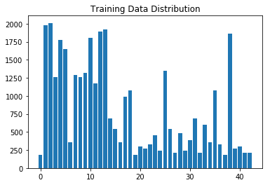
Here is an exploratory visualization of the data set. It is a bar chart showing the disturbution of different traffic sign in the train data set.
1. Describe how you preprocessed the image data. What techniques were chosen and why did you choose these techniques? Consider including images showing the output of each preprocessing technique. Pre-processing refers to techniques such as converting to grayscale, normalization, etc. (OPTIONAL: As described in the "Stand Out Suggestions" part of the rubric, if you generated additional data for training, describe why you decided to generate additional data, how you generated the data, and provide example images of the additional data. Then describe the characteristics of the augmented training set like number of images in the set, number of images for each class, etc.)
I tried two methods to process the image sets. One simple and fast and one complicated.
First method: I used np.power(image,0.65) to apply a Gamma correction to the RGB image.
This would enhance the darker images and make the contour stand out. And then I used np.dot with the weight of [0.2989, 0.5870, 0.1140]to change
the RGB image to grayscale. Last, I used (img-128)/128 to normalize the image.
Here is an example of a traffic sign image before and after grayscaling.
Second method I used exposure module from skiimage. I converted the RGB to grayscale using the same
method and normalize image by dividing it by 255. And then used exposure.equalize_adapthist to preform
Adaptive histogram equalization. However, this process takes about 6 mins to run on a single set of training data.
Although its output result look better and would improve our training, I have to use the method one
to save up the limited GPU time. Here is the image result from the exposure module:
From the histogram I created earlier, I decided to generate additional training images because certain class in the train set has less than 500 images. This would cause our model to be biased toward the classes that have higher number in the training data set.
To add more data to the the data set, I found this great code from https://github.com/vxy10/ImageAugmentation
to implement random distortion on images. I computed and stored all the sign classes, class indices and class count
from the label set y using np.unique. From every unique class, I create a random 50 indices within this class
and randomly pick from those indices again to select the exiting class image to feed into the transform_img, which would create a random distortion of the input image.
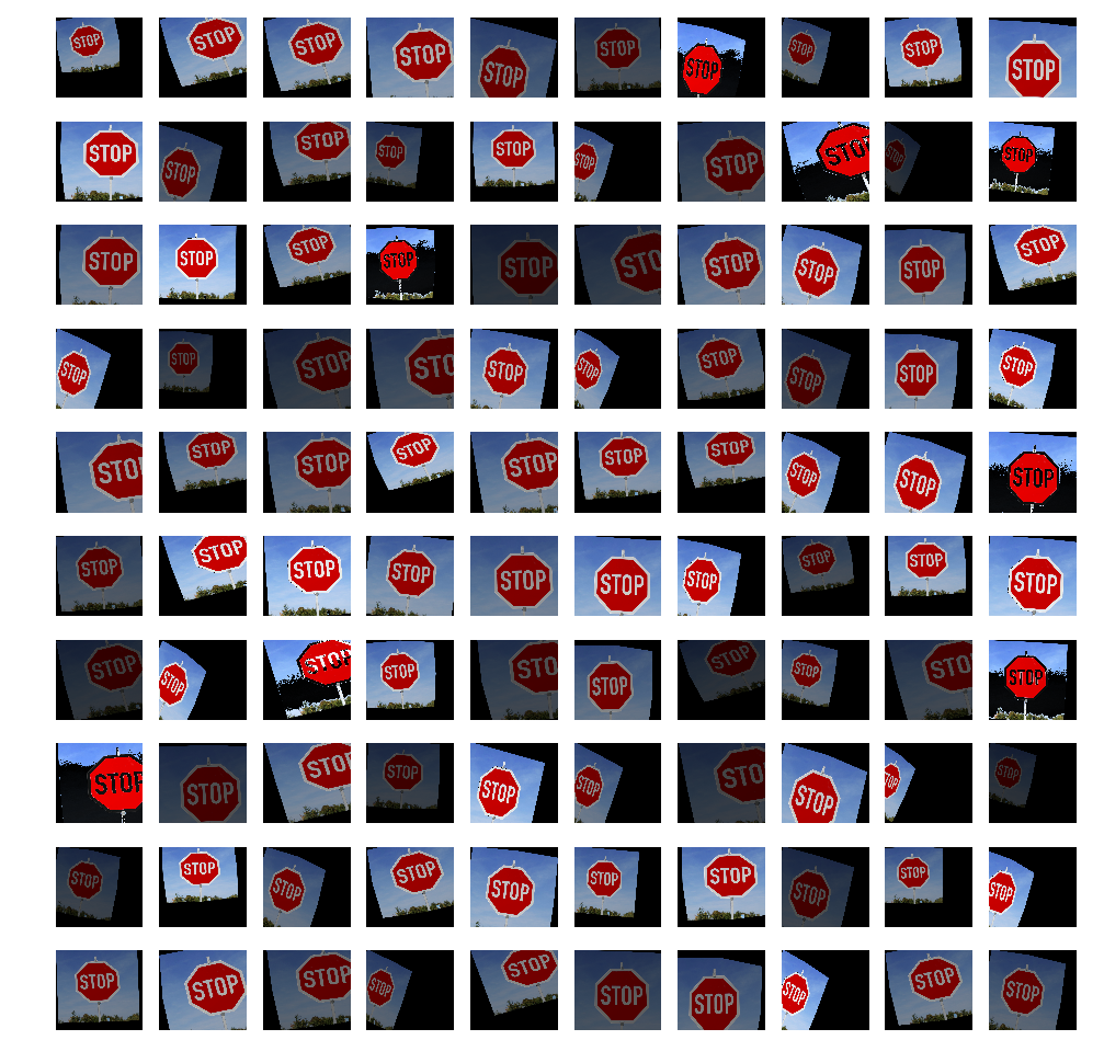
Below is the example of output of the transform_img from the vxy10
Once that is done, I sorted the lists I created to store all the new distorted images by index number in y label. I sorted those in a reverse order because later I would insert those new images into x data set from the end. During for loop operation, this method would not effect the the location of inserting index.
Here is an example of class 34 augmented images:
The augment data set follows a random transformation of rotation between -1 1 degree, translation of -1 and 1 and shear of -1 and 1. Note, I did observe that when the distoration is too big, the model would become under fitted due to the huge training images distortion.
2. Describe what your final model architecture looks like including model type, layers, layer sizes, connectivity, etc.) Consider including a diagram and/or table describing the final model.
My final model consisted of the following layers:
| Layer | Description |
|---|---|
| Input | 32x32x1 grayscale image |
| Convolution 5x5 | 1x1 stride, valid padding, outputs 28x28x16 |
| RELU | |
| Max pooling | 2x2 stride, outputs 14x14x16 |
| Convolution 5x5 | 1x1 stride, valid padding, outputs 10x10x32 |
| Max pooling | 2x2 stride, outputs 5x5x32 |
| Flatten | |
| Fully connected | weight 800x400 bias 400 |
| RELU | |
| Dropout | 0.75 keep |
| Fully connected | weight 400x200 bias 200 |
| RELU | |
| Dropout | 0.75 keep |
| Fully connected | weight 200x43 bias 43 |
| RELU |
3. Describe how you trained your model. The discussion can include the type of optimizer, the batch size, number of epochs and any hyperparameters such as learning rate.
To train the model, I used an learning rate of 0.0005, Epochs of 80 and batch size of 128
4. Describe the approach taken for finding a solution and getting the validation set accuracy to be at least 0.93. Include in the discussion the results on the training, validation and test sets and where in the code these were calculated. Your approach may have been an iterative process, in which case, outline the steps you took to get to the final solution and why you chose those steps. Perhaps your solution involved an already well known implementation or architecture. In this case, discuss why you think the architecture is suitable for the current problem.
My final model results were:
- training set accuracy of 99.7%
- validation set accuracy of 94.1%
- test set accuracy of 91.7%
If an iterative approach was chosen:
-
What was the first architecture that was tried and why was it chosen?
A: The first model I tried is the model from the previous lab, a classic LeNet. Two Covnets and two fully connected layers, with lower number of hidden layers. This gave me around 87% validation accuracy, which is a solid starting point.
-
What were some problems with the initial architecture?
A: The initial architecture would stop improving around epoch 15
-
How was the architecture adjusted and why was it adjusted? Typical adjustments could include choosing a different model architecture, adding or taking away layers (pooling, dropout, convolution, etc), using an activation function or changing the activation function. One common justification for adjusting an architecture would be due to overfitting or underfitting. A high accuracy on the training set but low accuracy on the validation set indicates over fitting; a low accuracy on both sets indicates under fitting.
A: Adding more layer of hidden layers of covnets and added one more layer of full connected was able to achieve a higher validation accuracy of 93% without using augment images to training set.
-
Which parameters were tuned? How were they adjusted and why?
A: I tried to increase the epoch size and lower the learning rate from 0.001 to 0.0005. Higher epoch size give the model more data to train. This increased the accuracy. Lower learning rate make the model train slower but when after awhile it would prevent overfitting of the model. However, if I lower the learnihng rate too much it would train the model too slow.
-
What are some of the important design choices and why were they chosen? For example, why might a convolution layer work well with this problem? How might a dropout layer help with creating a successful model?
A: When I used augmented images training set, the three layers of covnet become under fitted. The model would not train as fast and efficient as before. and the model become more likely to be underfitting. And then I reduce the model back to 2 layers of covnets and three fully connected layers to avoid underfitting. I tried the L2 regulation as well, adding beta and with L2 regulation to
optimizer.minimize. However, I don't see a big improvement on the accuracy I also adding dropout after the fully connected layers and after max pooling of the last covnet to reduce the overfitting during training, bring valid accuracy closer to the training accuracy.
1. Choose five German traffic signs found on the web and provide them in the report. For each image, discuss what quality or qualities might be difficult to classify.
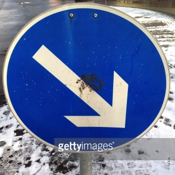
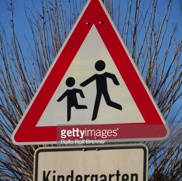
Here are five German traffic signs that I found on the web:
2. Discuss the model's predictions on these new traffic signs and compare the results to predicting on the test set. At a minimum, discuss what the predictions were, the accuracy on these new predictions, and compare the accuracy to the accuracy on the test set (OPTIONAL: Discuss the results in more detail as described in the "Stand Out Suggestions" part of the rubric).
Here are the results of the prediction:
| Image | Prediction |
|---|---|
| Keep Right | Keep Right |
| Children crossing | Children crossing |
| Road work | Dangerous curve to the left |
| Speed limit (60km/h) | Speed limit (60km/h) |
| Turn left ahead | Speed limit (60km/h) |
The first two images i have to resize them to 32x32. I used cv2.resize to reduce the image size.
The model was able to correctly guess 3 of the 5 traffic signs, which gives an accuracy of 60%. This compares favorably to the accuracy on the test set of 94% is low. This indicate our model is still bias toward curtain traffics. The augment of the data set might not be a good representation of the the real world image
3. Describe how certain the model is when predicting on each of the five new images by looking at the softmax probabilities for each prediction. Provide the top 5 softmax probabilities for each image along with the sign type of each probability. (OPTIONAL: as described in the "Stand Out Suggestions" part of the rubric, visualizations can also be provided such as bar charts)
For the first image, the model is relatively sure that this is a stop sign (probability of 0.6), and the image does contain a stop sign. The top five soft max probabilities were
| Probability | Prediction |
|---|---|
| 1 | Keep Right |
| .0 | Go straight or right |
| .0 | Turn left ahead |
| .0 | Yield |
| .0 | Dangerous curve to the right |
For the second image
| Probability | Prediction |
|---|---|
| 0.97 | Children crossing |
| .02 | Keep Right |
| .0 | General caution |
| .0 | Go straight or right |
| .0 | Speed limit (60km/h) |
For the third image, the prediction is completely wrong, does not even recognize the shape correctly
| Probability | Prediction |
|---|---|
| 0.44 | Speed limit (60km/h) |
| .26 | Dangerous curve to the left |
| .18 | Wild animals crossing |
| .08 | General caution |
| .01 | Speed limit (90km/h) |
For the Fourth image.
| Probability | Prediction |
|---|---|
| 0.96 | Speed limit (60km/h) |
| .02 | Road work |
| .01 | Right-of-way at the next intersection |
| .01 | No passing |
| .0 | Speed limit (90km/h) |
For the fifth image. This is also wrong.
| Probability | Prediction |
|---|---|
| 0.91 | Speed limit (60km/h) |
| .09 | Dangerous curve to the left |
| .00 | General caution |
| .0 | Speed limit (90km/h) |
| .0 | Slippery road |
In summary, my model does not have a well trained feature to recognize triangle and circle. This might caused by the reduce number of covnet. Having three of covnets could potentially improve recognition of shapes. In future practise and using local GPU setting, I would change back to three layers of covnet and have more hidden layers inside the covnet to have a more architecture to recognize shapes. I would also increase the epoch size to train the model if the model shows under fitting. Those tuning methods are only based on my experience on tuning model from this project. I would do more research on how other accomplished network to find out how others structure their network.


