scGCO is a method to identify genes demonstrating position-dependent differential expression patterns, also known as spatially viable genes, using the powerful graph cuts algorithm. ScGCO can analyze spatial transcriptomics data generated by diverse technologies, including but not limited to single-cell RNA-sequencing, or in situ FISH based methods.What's more, scGCO can easy scale to millions of cells.
This repository contains source codes of scGCO, and tutorials on running the program.
The primary implementation is as a Python 3 package, and can be installed from the command line by
pip install scgcoscGCO has been tested on Ubuntu Linux (18.04.1), Mac OS X (10.14.1) and Windows(Windows 7 Professional).
MIT Licence, see LICENSE file.
See AUTHORS file.
For bugs, feedback or help please contact Peng Wang wangpeng@picb.ac.cn.
The following codes demonstrate the typical data analysis flow of scGCO.
The tutorial has also been provided as a Jupyter Notebook in the Tutorial directory (scGCO_tutorial.ipynb)
The entire process should only take 1-2 minutes on a typical desktop computer with 8 cores.
The required matrix format is the ST data format, a matrix of counts where spot coordinates are row names and the gene names are column names. This default matrix format (.TSV ) is split by tab.
As an example, let’s analyze spatially variable gene expression in Mouse Olfactory Bulb using a data set published in Ståhl et al 2016.
from scGCO import *
import pandas as pd
import numpy as np
import matplotlib
import matplotlib.pyplot as plt
%matplotlib inline
import warnings
warnings.filterwarnings('ignore')- Step 1-5: perform genome-scale identification of spatially variably genes.
- Step 6-7: visualize and save identified spatial variably genes.
- Step 8: perform graph cuts on a single genes to visualize its spatial patterns.
j=11
unary_scale_factor=100
label_cost=10
algorithm='expansion'
ff = 'README_file/Rep'+str(j)+'_MOB_count_matrix-1.tsv'
locs,data=read_spatial_expression(ff,sep='\t',num_exp_genes=0.01, num_exp_spots=0.05, min_expression=1)

data_norm = normalize_count_cellranger(data)
print('Rep{}_processing: {}'.format(j,data_norm.shape))
raw data dim: (262, 16218)
Rep11_processing: (259, 12522)
exp= data_norm.iloc[:,0]
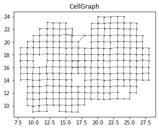
cellGraph= create_graph_with_weight(locs, exp)fig, ax= plt.subplots(1,1,figsize=(5,5)) #, dpi=300)
ax.set_aspect('equal')
exp= data_norm.iloc[:,0].values
cellGraph = create_graph_with_weight(locs, exp)
ax.scatter(locs[:,0], locs[:,1], s=1, color='black')
for i in np.arange(cellGraph.shape[0]):
x = (locs[int(cellGraph[i,0]), 0], locs[int(cellGraph[i,1]), 0])
y = (locs[int(cellGraph[i,0]), 1], locs[int(cellGraph[i,1]), 1])
ax.plot(x, y, color='black', linewidth=0.5)
plt.title('CellGraph')Text(0.5, 1.0, 'CellGraph')
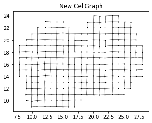
Both Mouse olfactor bulb and Breast cancer data sets used in the analysis have missing spots, creating holes in the grid. We recomment the users to fill the missing spot, and impute the missing values using AddPoints_XY_and_update_data function, for more accurate analysis results.
locs_new,data_norm_new,newPoints=AddPoints_XY_and_update_data(locs,data_norm,cellGraph,axis=1)
print('Filled {} points'.format(len(newPoints)))
print('After filled points: ', data_norm_new.shape)
Filled 6 points
After filled points: (265, 12522)
fig, ax= plt.subplots(1,1,figsize=(5,5)) #, dpi=300)
ax.set_aspect('equal')

exp_new = data_norm_new.iloc[:,0].values
cellGraph_new = create_graph_with_weight(locs_new, exp_new)
ax.scatter(locs_new[:,0], locs_new[:,1], s=1, color='black')
for i in np.arange(cellGraph_new.shape[0]):
    x = (locs_new[int(cellGraph_new[i,0]), 0], locs_new[int(cellGraph_new[i,1]), 0])
    y = (locs_new[int(cellGraph_new[i,0]), 1], locs_new[int(cellGraph_new[i,1]), 1])
    ax.plot(x, y, color='black', linewidth=0.5)

plt.title('New CellGraph')
Text(0.5, 1.0, 'New CellGraph')
t0=time.time()
gmmDict= multiGMM(data_norm_new)
print('GMM time(s): ', time.time()-t0)
100%|████████████████████████████████████████████████████████████████████████████████████| 8/8 [01:13<00:00, 9.15s/it]
GMM time(s): 74.15773129463196
# store_gmm(gmmDict,fileName='')t0= time.time()
result_df= identify_spatial_genes(locs_new, data_norm_new,
cellGraph_new ,gmmDict)
print('Running time: {} seconds'.format(time.time()-t0))100%|████████████████████████████████████████████████████████████████████████████████████| 8/8 [01:51<00:00, 13.97s/it]
Running time: 112.93512773513794 seconds
The results of scGCO can be saved to .csv files using write_result_to_csv function.
And the saved .csv file can be accessed using read_result_to_dataframe function.
write_result_to_csv(result_df,'../../results/MouseOB/scGCO_results/Rep{}_results_df'.format(j))result_df=read_result_to_dataframe('../../results/MouseOB/scGCO_results/Rep11_result_df.csv')
print(result_df.shape)(12522, 269)
- default: 0.05
select genes demonstrating significant spatial variability
fdr_cutoff=0.05
fdr_df=result_df.sort_values('fdr').loc[result_df.fdr<fdr_cutoff,]

print(fdr_df.shape)
(333, 269)
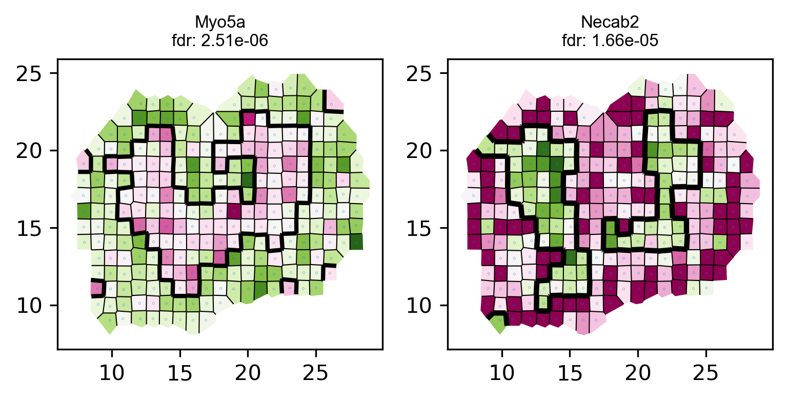
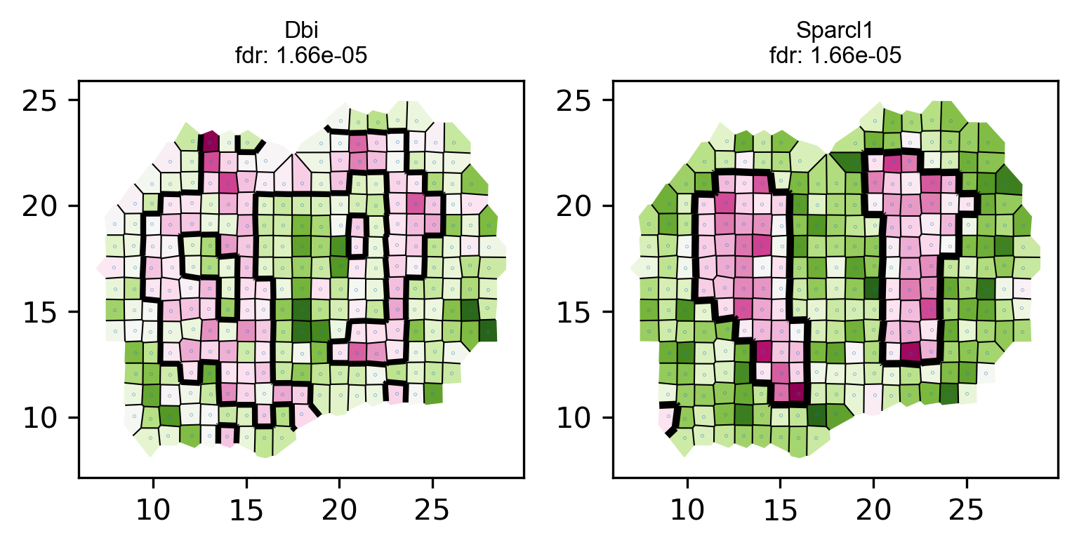
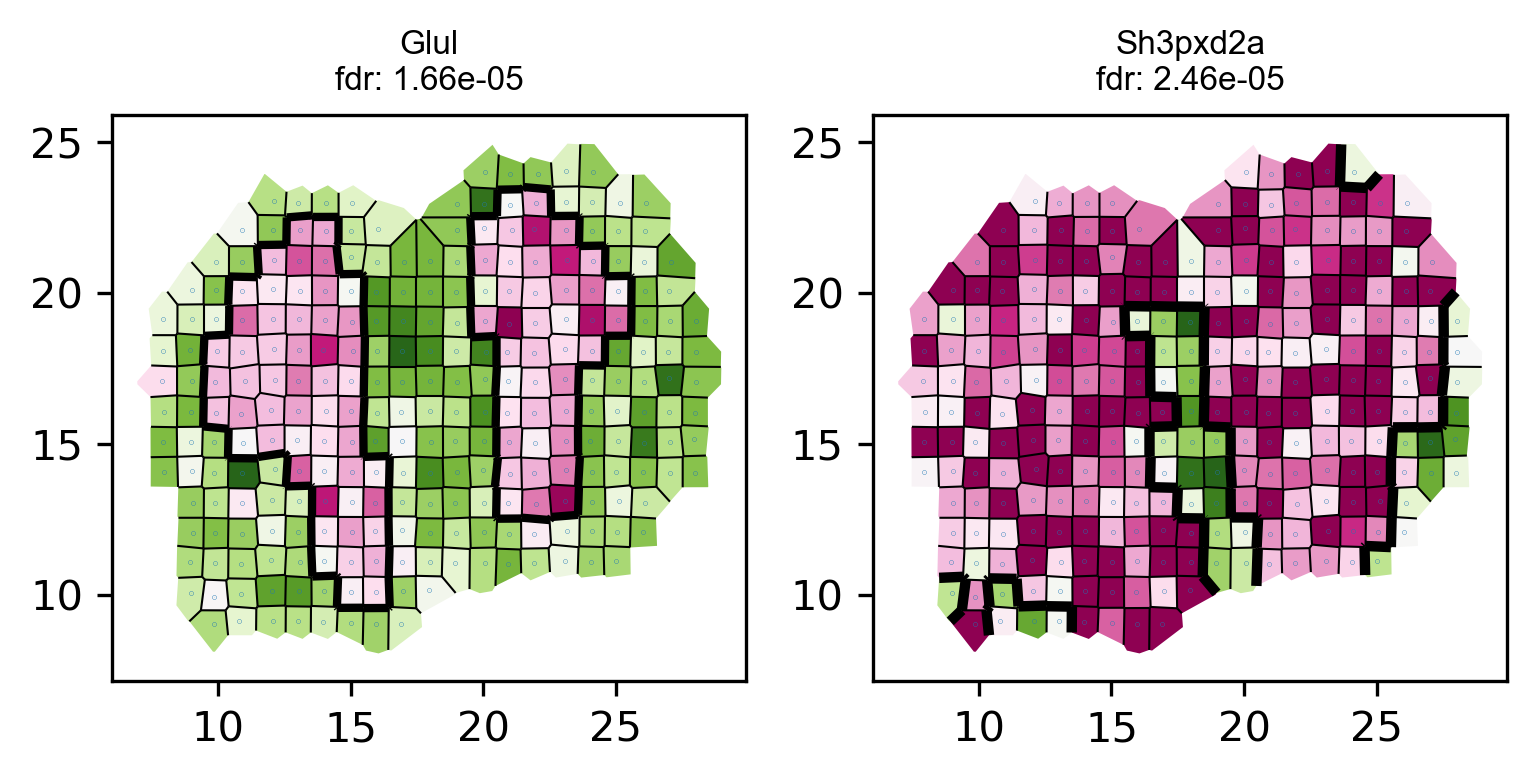
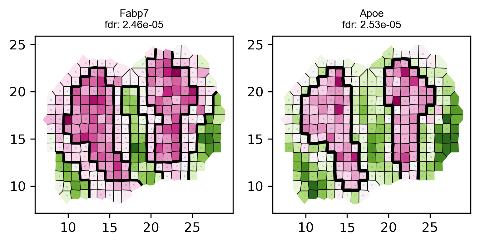
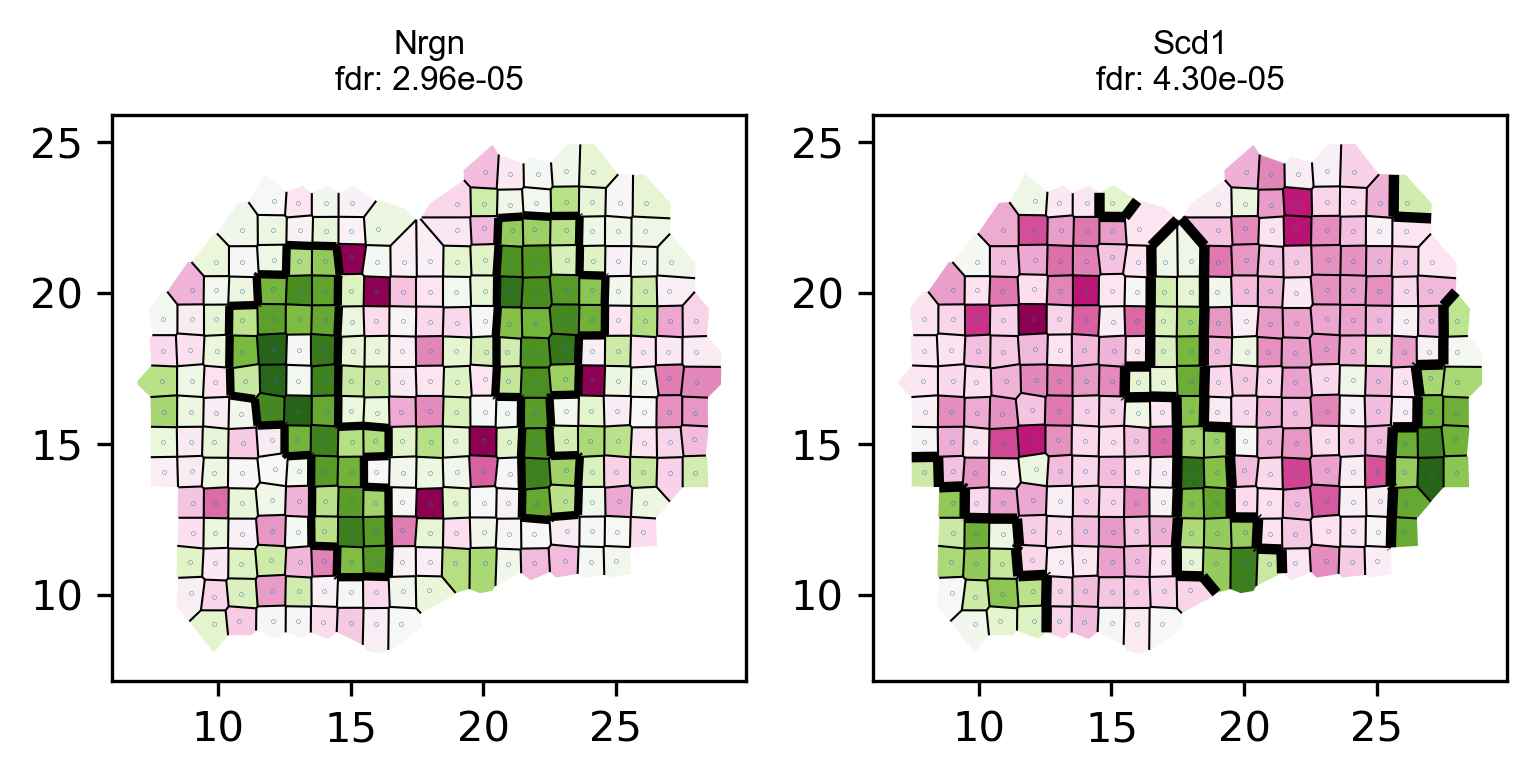
Visualize some identified genes.
# visualize top genes
visualize_spatial_genes(fdr_df.iloc[0:10,], locs_new, data_norm_new ,point_size=0.2)
# save top genes to pdf
multipage_pdf_visualize_spatial_genes(fdr_df.iloc[0:10,], locs_new, data_norm_new,point_size=0) #,
# fileName='../../results//top10_genes.pdf')
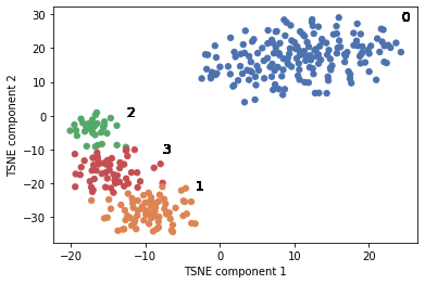
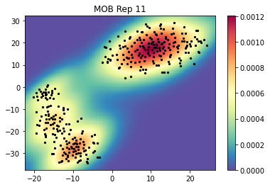
Perform t-SNE and visualize the clustering of identified genes.
marker_genes = ['Pcp4','Apod','Slc17a7','Glul']
tsne_proj_df = spatial_pca_tsne_kmeans_cluster_gene(data_norm_new,
                                                    fdr_df.index,
                                                    marker_genes,
                                                    perplexity = 30,
                                                    fileName=None)
# plot_tsne(tsne_proj_df.iloc[:,0:2].values,tsne_proj_df.iloc[:,2]) #,
# fileName='../../PDF_file/supple_figure/Fig2b.pdf')fig,ax = plt.subplots()
zz=visualize_tsne_density(tsne_proj_df.iloc[:,0:2].values,title=title,bins=200,threshold=0.1,ax=ax,fig=fig)
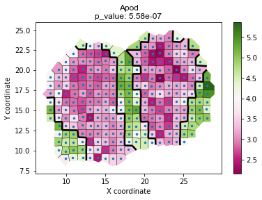
Perform graph cuts for a single gene.
# You can also analyze one gene of interest

geneID='Apod' # Lets use Nrgn as an example
unary_scale_factor = 100 # scale factor for unary energy, default value works well
label_cost=10
algorithm='expansion'
# set smooth factor to 20 for example;
# use bigger smooth_factor to get less segments
# use small smooth_factor to get more segments
smooth_factor=20

ff = '../../data/Raw_data/MOB-breast_cancer/Rep11_MOB_count_matrix-1.tsv'
# read in spatial gene expression data
locs, data = read_spatial_expression(ff,sep='\t')

# normalize gene expression
data_norm = normalize_count_cellranger(data)

# select anyone gene's expression
exp =  data_norm.iloc[:,0]

# create graph representation of spatial coordinates of cells
cellGraph = create_graph_with_weight(locs, exp)

## Fill spots
locs_new,data_norm_new,newPoints=AddPoints_XY_and_update_data(locs,data_norm,cellGraph,axis=1)

# recreate new cellGraph after filled sopts.
exp_new =  data_norm_new.iloc[:,0]
cellGraph_new = create_graph_with_weight(locs_new, exp_new)


# GMM
count = data_norm_new.loc[:,geneID].values
gmm=perform_gmm(count)

# do graph cut
temp_factor=smooth_factor
newLabels = cut_graph_general(cellGraph_new, count, gmm, unary_scale_factor,
                                           temp_factor, label_cost, algorithm)
# calculate p values
p, node, com = compute_p_CSR(locs_new, newLabels, gmm, count, cellGraph_new)

# Visualize graph cut results
plot_voronoi_boundary(geneID, locs_new, count,  newLabels, min(p))
raw data dim: (262, 16218)
/ [root]
├── code
│   ├── scGCO_code
|         ├── scGCO # the source code folder for running scGCO
|   ├── analysis
|   |        ├── FIG2_a_b_c_d.ipynb:this notebook will reproduce main figure2a_2b_2c_2d
|   |        ├── FIG2_e_f.ipynb:this notebook will reproduce main figure2e_2f
|   |        ├── Simulation
|   |               ├── notebooks : this folder contains simulation scripts and runing scripts
|   |               ├── processed_data : this folder contains sim_mob sample info, tissue mat and simulation counts
|   |               ├── compare : this notebook will reproduce Suppl Figure6
|   |                    └── gen_Supple_Fig1.ipynb : this notebook will reproduce Suppl Figure1
|   |        ├── MouseOB
|   |               ├── Supple_Fig3_tsne_Genes_cluster_MOB.ipynb : this notebook will reproduce Suppl Figure3
|   |               ├── Supple_Fig4-markGenes-Rep9.ipynb : this notebook will reprodece Suppl Figure4
|   |               ├── Supple_Fig8-Tissue_structure.ipynb : this notebook will reproduce Suppl Figure8
|   |                    └── ...
|   |        ├── Breast_Cancer
|   |               ├── Supple_Fig12-Breast cancer.ipynb : this notebook will reproduce Figure2_e_f and Suppl Figure12
|   |        ├── MERFISH
|   |               ├── Supple_Fig15-MERFISH.ipynb : this notebook will reprodece Suppl Figure15
│   ├── Computation-Performance
|         ├── Fig2g_Compare_memory_simulation_data.ipynb # this notebook is for comparing occpuied memory of three three methods and shown in main fig2g
|         ├── Fig2h_Compare_time_simulation_data.ipynb # this notebook is for comparing running speed of three three methods and shown in main fig2h
|   |     ├── Simulate_script
|                   ├── create_performance_bigdata_R.ipynb # the code is for millions simulate data
|                   ├── scGCO_performance_run.ipynb # the code is for testing scGCO running speed and occupied CPU memory with simulate data

|                   ├── SPARK_performance_run.R # the code is for testing scGCO running speed and occupied CPU memory with simulate data
|                   ├── spatialDE_simulate_script.ipynb # the code is for testing spatialDE running speed and occupied CPU memory with simulate data
│   ├── README.md
|
├── data
|   ├── HighVariableGenes
|           ├── [Rep11_MOB seruat results  Tepe_MOB_hvg]
|   ├── MOB_DESeq2_results
|           ├── [Rep11 clustering 5 Layers and DESeq2 results]
|   ├── Performance_BigData
|           ├── [1M_cells_100genes_counts]
|   ├── HighVariableGenes
|           ├── [All datasets seruat results]
|   ├── Raw_data
|           ├── [All datasets counts data and HE image]
└── results
|    ├── Figure
|    |        ├── Figure2.pdf # Figures that were output by execution of the notebook
|    |        ├── Suppl_Fig2.pdf
|    |        └── ...
|    ├── MouseOB # Notebooks that have been pre-compiled with nbconvert
|    ├── BreastCancer
|    └── ...
└── Temp_files
|    |        ├── Rep11_scGCO_tsne_proj_df # DataFrame that were used in execution of the notebook
|    |        ├── data_norm_new
|    |               └── ...
|    |        └── tissue_mat
|    |               └── ...
Several Jupyter Notebooks are provided in the analysis directory to reproduce figures of the paper.
Several Jupyter Notebooks are provided in the Computation-Performance directory to reproduce the running time simulation results reported in the main text.
- Compare_memory_simulation_data.ipynb: This notebook generates Fig. 2g using precomputed data.
- Compare_time_simulation_data.ipynb: This notebook generates Fig. 2h using precomputed data.
This script takes about 20 hours to finish on a typical 8 cores computer.
