MSCKF Tutorial

Introduction

This project contains a basic Multi-Constraint Kalman Filter(MSCKF) implementation to solve the visual inertial odometry(VIO) problem. The MSCKF is an extended kalman filter first introduced in "A Multi-State Constraint Kalman Filter for Vision-aided Inertial Navigation" by Mourikis and Roumeliotis, and is the main way to solve VIO within the EKF framework.

This project should serve as a tutorial. Hopefully, people can read through the codebase and learn how an MSCKF works. It is a fairly basic implementation, and lacks some of the more modern upgrades such as the observability constraints. Plus as it is implemented in Python it lacks the speed necessary to run this on a actual system. If you do want a useful, performant MSCKF solution then I recommend the OpenVINS project.

Getting Started

Installation

The project is developed with poetry to control the dependencies. If possible I recommend to setup the project using it, and run the commands with it.

Poetry setup

Activate your poetry environment and run poetry install in the msckf_tutorial folder. You can now run the examples by prepending your commands with poetry run.

Python Virtual environment setup.

It is assumed you already have setup, or can setup a python virtual environment.

Install the project to your virtualenv. I recommend using pip install -e ..

Running examples.

Download one of the runs from the Euroc dataset in the ASL format, and unzip the compressed file.

Run the VIO algorithm using the following command

python ./examples/run_on_euroc.py --euroc_folder <PATH_TO_MH2_MAV0> --use_viewer --start_timestamp 1403636896901666560

The start_timestamp is needed right now as we don't run an initialization scheme, and Euroc has some drastic movement in the beginning to initialize the system. It should be set to timestamp where the drone is about to take off after the bias initialization movement. Here the value 1403636896901666560 is for the MH02 run.

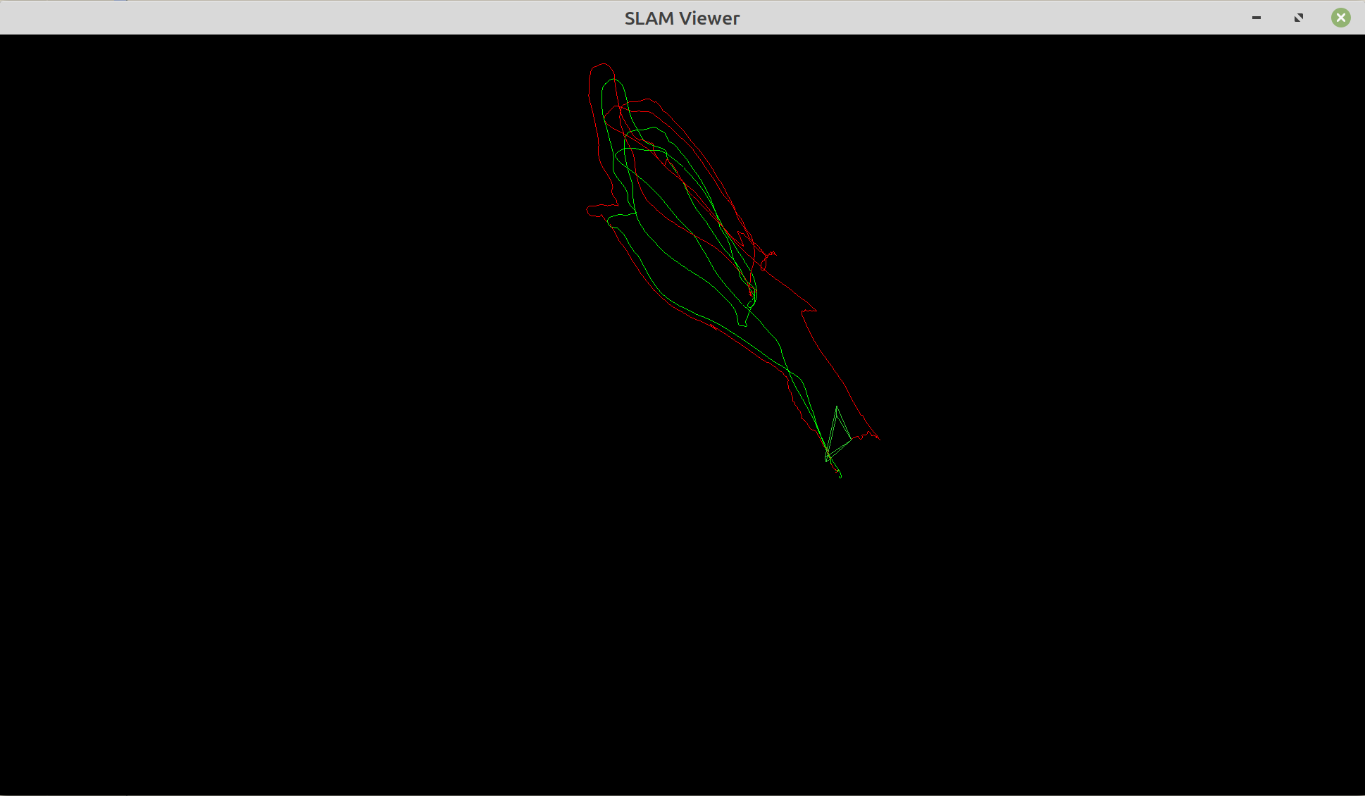
If you add the --use_viewer option a window should pop up which draws the current camera pose and the trajectories. Green is the ground truth, and red is the estimated one. You can control the movement of the camera with WASD keys.

Primer on Transforms and Notation

This assumes you already have a basic understanding of rotations, and transforms.

Basic homogenous transforms.

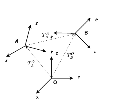
In the above image you can see 3 coordinate system which we will call Frame A and Frame B and O(for origin). They are related to each other by a rigid body transform( $T$ ). Which is composed of a rotation $R$ and a translation $t$ .

We generally mark our transforms with the coordinate frames.

$T_B^A$ Which can be read as either
- The transform of Frame B in Frame A
- The transform from Frame A to Frame B.
$R_B^A$ same thing for rotation, and translation $t_B^A$ .

The simplest way to represent our Transform( $T$ ) is with a 4x4 homogenous matrix.

$\begin{bmatrix}R & t\\ 0_3 & 1\end{bmatrix}$

This has the advantage multiple advantages:

We can chain together transforms with matrix multiplication.
- $T_A^O*T_B^A=T_B^O$
The matrix inverse is equivalent to the transform inverse.

$T^{-1}=\begin{bmatrix}R & t\\ 0_3 & 1\end{bmatrix}^{-1}$

We can represent a 3D point as a homogenous vector $[x,y,z,1]$ and are able to transform it with matrix vector multiplication.

Quaternions

An alternative to the homogenous transform is to store the rotation as a quaternion. Our transform is then just a pair of the quaternion and rotation, and is equivalent to the homogenous transform. $(q,t)=\begin{bmatrix}R & t\\ 0_3 & 1\end{bmatrix}$

All the operations discussed above with homogenous transform are possible with the quaternion translation pair. You just have to change certain matrix operations to their quaternion equivalent.

For an in depth tutorial on Quaternions I recommend the paper Quaternion kinematics for the error-state Kalman filter by Joan Solà, which also discusses how to implement the operations.

Notation in code

In the code the notation is as follows.

frame1_X_frame2

Frames 1,2 can be changed to the actual name of coordinate frames(e.g camera,imu,body,world,...) X represents some sort of transformation object(e.g T for Transform, R for rotation, t for translation,...). It stands for the transform object that transforms Frame 1 into Frame 2.

An example would be:

$T_C^I$

imu_T_camera

The transform of the imu frame to the camera frame.

The advantage of this notation is that it allows you to check if two transform objects are even allowed to be composed together.

Let's imagine we have a point in the camera frame which we want to transform into the imu frame. In code this would look like so:

pt_in_imu = imu_T_camera * pt_in_camera

here we can see that this is valid as the camera parts of the names are adjacent.

An invalid example would be:

pt_in_imu = camera_T_Imu * pt_in_camera

Here we have a pt_in_camera adjacent to imu so we know we have a problem.

Note that this also works with almost all the transform objects.

global_T_camera = global_T_imu * imu_T_camera

Here is a table of all the transformation quantities you can find in the codebase.

Symbol	What is represents
T	Rigid Body Transform as a 4x4 homogenous matrix
R	3x3 Rotation Matrix
t	translation
Q	Hamiltonian Quaternion
JPLQ	Quaternion in the JPL style
JPLPose	A rigid body transform stored as a jpl quaternion and translation pair

MSCKF differences

In most literature and in this project you will find that the MSCKF works differently in how it handles rigid body transforms. The most significant being the use of the jpl style quaternions, and that they store the rotation in the opposite direction compared to most people.

JPL style Quaternions.

Storage of rotation.

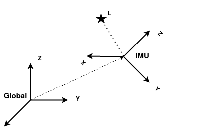
In VIO we are trying to estimate the pose of the IMU frame in some global coordinate system.

In most cases the exact transform we are trying to estimate can be written as $T_I^G$ . It is possible to store it as a homogenous transform, but generally we store the rotation and translation separately as a pair $[R_I^G,t_I^G]$ . We also generally use quaternions as our rotation representation so it should look like so $[{}_hq_I^G,t_I^G]$ where ${}_hq$ marks it as a hamiltonian quaternion. This is equivalent to the homogenous matrix $\begin{bmatrix}R_I^G & t_I^G\\ 0_3 & 1\end{bmatrix}$ .

MSCKF Style

The MSCKF stores the inverted rotation matrix of our above format. So instead of the pair $[R_I^G,t_I^G]$ it instead stores $[R_G^I,t_I^G]$ where $[R_G^I]$ is the rotation of the global frame in the IMU frame. In addition it uses a JPL style quaternion to represent the rotation $[{}_{j}q_G^I,t_I^G]$ . This means our pair is no longer equivalent to the standard homogenous matrix, and is instead equal to $\begin{bmatrix}R_G^I & -R_G^It_I^G\\ 0_3 & 1\end{bmatrix}$ .

References

A. I. Mourikis and S. I. Roumeliotis, "A Multi-State Constraint Kalman Filter for Vision-aided Inertial Navigation," Proceedings 2007 IEEE International Conference on Robotics and Automation, 2007, pp. 3565-3572, doi: 10.1109/ROBOT.2007.364024.

A. I. Mourikis and S. I. Roumeliotis, "A Multi-State Constraint Kalman Filter for Vision-aided Inertial Navigation," University  of  Minnesota,  Dept.  of  Comp.  Sci.& Eng., Tech. Rep

N.  Trawny  and  S.  I.  Roumeliotis,  “Indirect  Kalman  filter  for  3D attitude  estimation,”  University  of  Minnesota,  Dept.  of  Comp.  Sci.& Eng., Tech. Rep., Mar. 2005

Joan Solà "Quaternion kinematics for the error-state Kalman filter" https://arxiv.org/abs/1711.02508

Frank L. Lewis, Lihua Xie, Dan Popa " Optimal and Robust Estimation With an Introduction to Stochastic Control Theory Second Edition"

Richard Hartley, Andrew Zisserman "Multiple View Geometry in Computer Vision"

Edwinem/msckf_tutorial