Repository for the homework of Image Analysis and Computer Vision course of Politecnico di Milano 2017/2018.
- src: The principal matlab files are inside the "src" folder. The folder "old" inside "src" contains old matlab files.
- reference: contains reference documents useful during the development.
- doc: contains the assignments and the documentation of the project
- matlab_output: contains output data
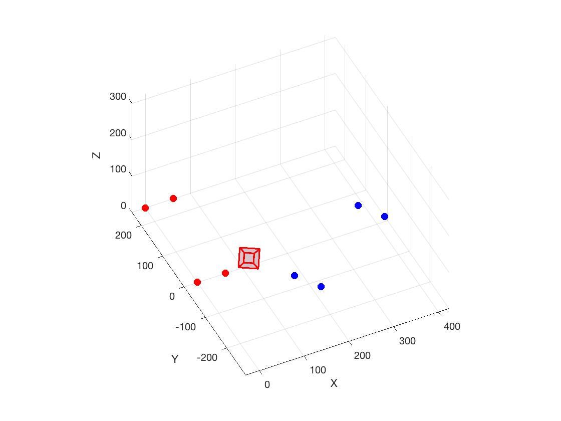
The main matlab file is "main.m" that contains all the workflow. The variable debug must be true if the user wants to see all the images generated during the algorithm. If the variable auto_selection is true the lines hardcoded are used. If false the lines must be selected manually from the user. During the line selection phase the user must read the title of each image in order to select lines in appropriate way. To select a line the user must select a point near the line. There are four methods for Camera Calibration, the user can select the most appropriate one (the one with all constraints, i.e. the last one, probably is slightly better than the other). In the camera localisation images the left horizontal face is identified with red points, while the right horizontal face with blue points. Points on the vertical faces can be selected through line intersection or through manual selection of points. In both cases points are green.
The folder "matlab_output" contains the output data of matlab, generated using the diary function. Files starting with k are the calibration matrices obtained with different constraints:
- k.txt is the matrix with only the line at infinity constraints and the homography constraints
- k_vp_n.txt is the matrix obtained with only normalised vanishing points orthogonality constraints
- k_vp_nn.txt is the same as before but with vanishing points not normalized
- k_all.txt is the calibration matrix obtained with all constraints normalised
- out.txt contains all the data from a run of the algorithm
- results.mat contains the results inside out.txt in matlab format
For more details please refer to the documentation.
The folder images contains images generated during the algorithm.
- Input_image: original input image
- edges: extracted edges
- lines: extracted lines
- affine_rectification: the affine rectified image
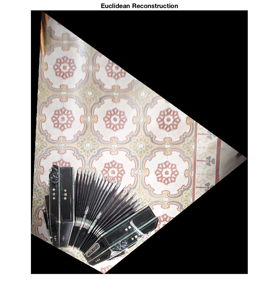
- shape_reconstruction: shape reconstruction of the horizontal plane
- cam_loc_l/cam_loc_l2/cam_loc_l3: camera localisation wrt the left horizontal face
- cam_loc_r/cam_loc_r2/cam_loc_r3: camera localisation wrt the right horizontal face
- cam_loc/cam_loc2/cam_loc3: camera localisation wrt the both horizontal faces
- vertical_face_left: shape reconstruction of the left vertical face
- vertical_face_right: shape reconstruction of the right vertical face
- hor_sr_l_using_P: shape reconstruction of horizontal plane using the pinhole model with the world on the left horizontal face
- hor_sr_r_using_P: shape reconstruction of horizontal plane using the pinhole model with the world on the right horizontal face
- 3d_shape_rec/3d_shape_rec2: coordinates of the 3d shape reconstruction of the object
A bandoneon is a musical instrument, consisting in two rigid wooden parts connected by a deformable bellow. The assignment is to reconstruct the bandoneon shape from a single image of it, using additional information. In the given image, the bandoneon is placed on a horizontal floor. Four rectangular faces are visible in the image: two coplanar horizontal faces, and two non-coplanar vertical faces. The long side of the horizontal faces is 243 mm, and it is slightly longer than the long side of the vertical face. For each horizontal face, two groups of parallel lines can easily be identified. The two groups of lines are mutually perpendicular. One of the (short) lines on each horizontal face is also common to a vertical face. Part of the horizontal floor is also visible: we can assume to see groups of parallel lines (the groups are also mutually orthogonal): These lines can be used to help in robustly find, e.g., the image of the horizontal vanishing line (i.e. the image of the line at the infinity of the horizontal plane). We can NOT assume square patterns on the floor. In addition, the long lines in the vertical faces are vertical (i.e. orthogonal both to the horizontal faces and to the floor).
- Image feature extraction and selection: Use the learned techniques to find edges and lines in the image. Then manually select those lines which are useful for the subsequent steps.
- Geometry 2.1 Using constraints on the horizontal lines, and their images, reconstruct the shape of the horizontal faces, and determine their relative position and orientation. 2.2 Using also the images of vertical lines, calibrate the camera (i.e., determine the calibration matrix K) assuming it is zero-skew (but not assuming it is natural). See the Hint reported below. 2.3 Localize the camera with respect to (both) horizontal faces. From the image of the (short) horizontal segments common to a horizontal face and its neighboring vertical face, reconstruct the shape of the vertical faces
Here we used a stratified approach to shape reconstruction.
The final result should be an image such that the transformation between the real scene and the image is a similarity.
In order to perform affine rectification we require that the line at infinite in the image is mapped back to itself.
So we first perform the identification of the imaged line at infinite through LSA using 10 couples of imaged parallel lines.
Once found the image of the line at infinite the reconstruction matrix that rectifies the image it's simple.
The last row is the imaged line at infinite.
[pag 49 Multiple View Geometry in computer vision]
Once the image has been affinely rectified we have obtained an image such that the transformation from the original scene is an affine transformation.
Notice that the Upper left part is a symmetric matrix and homogeneous, so it has only 2 DOF.
So we can use two pair of orthogonal lines to determine its parameters.
Once found C_star_inf_prime we can use standard cholesky (or SVD) to determine Ha.
Once we have reconstructed the shape of the object metric properties can be determined, like angles.
The relative orientation between vertical faces can be determined using the cosine between the two lines representing the longest line.
The relative position can be determined simply by computing the difference between the origin of the two reference frames and multiplying by the scaling factor.
Camera calibration is determining the matrix K:
P=[KR | -KRo]
Where R is the Rotation between the camera and the world and o is the location of the camera wrt the world reference frame.
In order to determine K we need to specify some constraints on Omega (the image of the absolute conic).
Here we can use the homography method (p 211 Multiple View Geometry in Computer Vision) adapted with the reconstructive transformation (that we have found in the previous point) on the horizontal faces.
-
For each horizontal face we can compute the transformation that maps its corner points to their imaged points (H_r^-1 since H_r maps the image point to their real shape).
-
We can compute the imaged circular points for the plane of that face as H_r(1,+- i, 0)'. Writing H = [h1, h2, h3], the imaged circular points are h1 +- ih2.
-
This gives us two constraints on the image of the absolute conic since the circular points lie on omega:
Which are linear equations in omega.
Other constraints that can be used are the constraints deriving from the fact that the line at infinite on the horizontal plane is orthogonal wrt the vanishing points on the vertical direction on the vertical face:
[l_inf]x * omega * v_p = 0
Where [l_inf]x is the vector product matrix of l_inf. In order to determine the vanishing point of the vertical direction we can use a least square approximation using all vertical lines on the vertical face.
In this point we have to find the relative position of the camera wrt the reference frame placed on the horizontal faces.
This is possibe knowing the shape of the horizontal faces, knowing the size, knowing the image and knowing K.
The main formula is:
[i, j, o] = K^-1 *H
Where H is the transformation mapping world points to image point. In this case it's H_r^-1 * H_omog^-1.
H_omog it's easy to find since knowing the rectified image we should only impose it's real measure.
H_omog transforms the rectified image in the real world scene.


