Instructions and scripts for running different Genome-Wide Association Scans (GWAS)
is a
software package that can run several variations of the Mixed Model
Algorithm.
GEMMA will accept a couple of different input formats; the easiest one the generate is the Plink bed/bim/fam format, because there are already several existing programs that can convert between this and other common formats.
If you do not have it already, download and install
.
If you are starting with a VCF file, then the command to convert it into bed/bim/fam format will look like this:
plink --vcf <yourFilename> --make-bed --allow-extra-chr --out <newFilename>If you are starting with a HapMap file, such as those created by
, then you will need a
couple of extra steps.
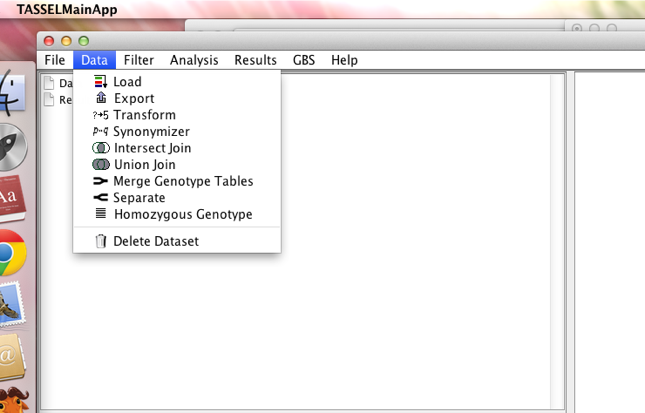
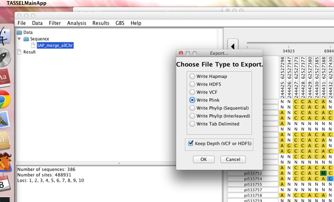
First, load your HapMap file into the TASSEL alignment viewer. Then, use the export option to write your files out into Plink format.
This will create 2 files: a .ped and a .map file. Both files
should have the same prefix. Now, you can use these files in Plink
with the make-bed command:
plink --file <plink-file-prefix> --make-bed --allow-extra-chr --out <newFilename>After you have run Plink, you will have 3 files with the same prefix: .bed, .bim, and .fam. The .fam file is the one that will need to contain the phenotypes; you will need to manually edit this file to add your phenotype data.
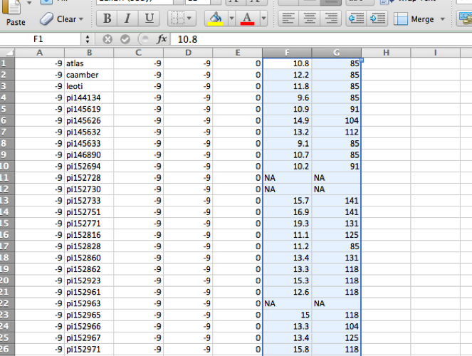
The starting .fam file should contain 6 columns (you can open this
file in Excel as a .txt file, or in R as a table). At this point,
the 6th column will contain all "-9" values, which stands for missing
data. Insert your phenotypes starting at Column 6, and adding as many
additional columns as you want.
Save the edited file as a tab-delimited txt file. You can rename this
back to a .fam file from the command line: mv file.txt file.fam
Also note that you may need to run mac2unix or dos2unix to get rid
of special line ending characters, depending on what program you used
to edit.
Once you have installed GEMMA and generated your input files, you should be able to run the program according the the GEMMA users manual.
Below are instructions for a couple of variations on running GEMMA in the LMM and BSLMM modes, where you may need to generate or process additional files.
While GEMMA has internal programs for calculating kinship, you may want to run the Linear Mixed Model (LMM) with external estimations of population structure.
In this example, I generate a PCA matrix using Plink, adjust the format with some simple bash commands, and then incorporate it into a GEMMA command line.
- Using Plink to run PCA. The key thing to remember here is to make sure the number of principal components that Plink reports is equal to the number of samples in your file (because GEMMA requires this). So, if I have a sample of 100 individuals:
plink --pca 100 --file <your-plink-prefix> --out <output-pca>- Getting rid of the first 2 columns with the command line. Plink will create 2 files: a .eigenvec and a .eigenval file. You will need both, but the .eigenvec file needs to be edited a bit.
awk '{$1="";print}' output-pca.eigenvec | awk '{$1="";print}' >>new.eigenvec- Running GEMMA:
gemma -bfile <your-file-prefix> -n 1 -d <output-pca.eigenval> -u <new.eigenvec> -lmm 4 -o <your-output-name>The command line for running a single iteration of the BSLMM (the Bayesian Sparse linear mixed model):
gemma -bfile <your-file-prefix> -bslmm 1 -n 1 -w 5000000 -s 20000000 -o <your-output-name>The n 1 flag tells the program to look at the first phenotype in the
file; the -w 5000000 is telling it to perform 5 million burn-in
runs, and the -s 20000000 tells it to do 20 million sampling steps.
Because you want to make sure Bayesian models aren't getting stuck on local maxima, it is a good a idea to do multiple independent runs (10 separate runs is a good number to ensure convergence).
After getting all 10 runs to finish, you can combine results and get
the parameter means with the code contained
Rcode_analyze_BSLMM_means_across_chains.R.
You will need to edit this code to contain your file paths and file names. Also, this script was originally written by Aaron Comeault, so if you use it please cite: Comeault, A.A. et al. (2015) Selection on a Genetic Polymorphism Counteracts Ecological Speciation in a Stick Insect. Current Biology 25(15):1975-1981.
is a tool written specifically
for R that can also implement several mixed models (although it cannot
perform the Bayesian model).
GAPIT expects the genotype data to be in the HapMap format used by TASSEL. If your data are in another format, it is possible you can still read them into the TASSEL alignment viewer and use the export function to create hapmap files.
If you data are in a format that cannot be read by TASSEL, you will need to convert them yourself.
Your phenotype data should be in a separate .csv or .txt file.
This file needs to have the first column be named "Taxa" and contain
all of your sample names. Then, each column after that should contain
phenotype data. You can have as many phenotype columns as you want;
GAPIT will automatically run through them all.
The code to run GAPIT is very simple, and can be found in
Gapit_Rcode.R.
After running GWAS, you will likely want to see what genes are closest to your significant SNPs.
To do this, you will need to obtain an annotation file (.gff3) for your reference genome, along with an "annotation-info" file that contains the descriptions associated with each gene ID. These types of files can be downloaded from Phytozome, UCSC Genome Browser, Ensembl, or wherever you got your reference genome file.
You can use the R code in geneScan_topSNPs.R to find the code for a
function to scan for nearby genes and match them up to their descriptions.


