Surface reconstruction library and CLI for particle data from SPH simulations, written in Rust.
This repository consists of the following crates:
- 🛠️
splashsurf: Binary crate with a CLI (command line interface) to quickly run surface reconstructions of SPH particle data files from the terminal. Install withcargo install splashsurf. - 🧰
splashsurf_lib: Library that implements the reconstruction pipeline used by the CLI. Allows integrating the reconstruction procedure directly into other Rust applications. Furthermore, it resembles a framework providing access to individual building blocks to create your own surface reconstruction pipeline. - 🐍
pysplashsurf: Bindings to the CLI and library for Python. Install withpip install splashsurfand see theREADMEfor more details.
This page provides an overview of the CLI's features and high-level notes on implementation of the reconstruction method.
splashsurf is a tool to reconstruct surfaces meshes from SPH particle data.
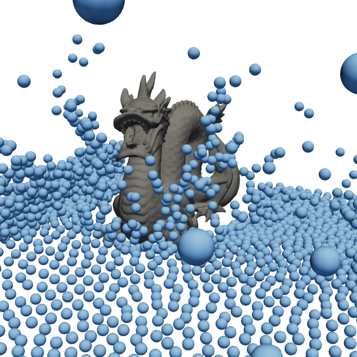
The first image shows the visualization of a set of particles from an SPH fluid simulation from SPlisHSPlasH.
The particle radius is 0.025. As the rendering of a fluid should not look like a ball pit, a surface mesh has to be
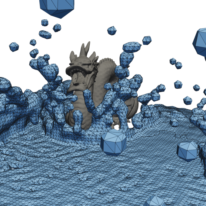
reconstructed from this particle data. The next image shows a reconstructed surface mesh of the fluid produced by splashsurf
with a "smoothing length" of 2.2 times the particles radius and a cell size of 1.1 times the particle radius. The
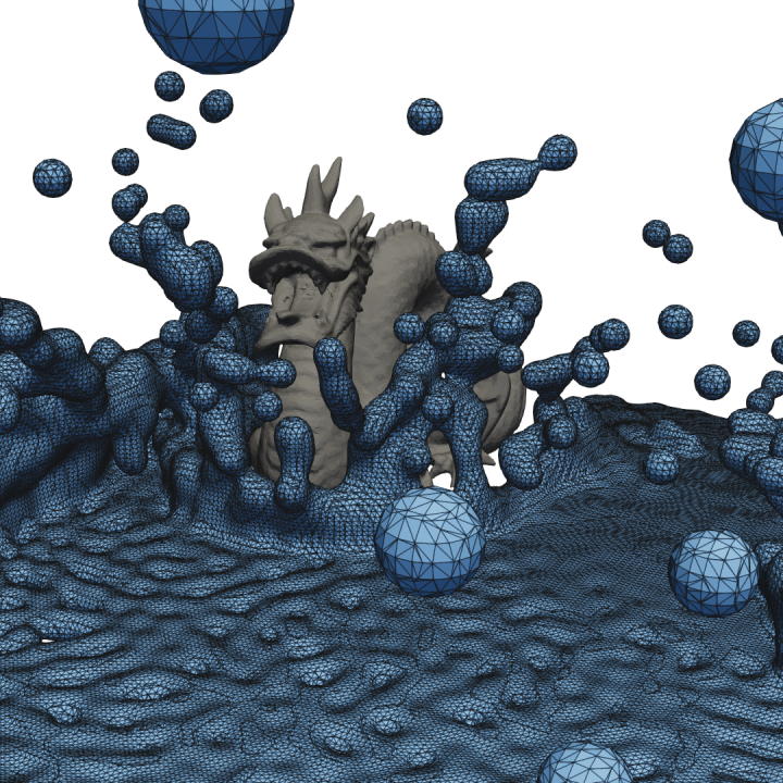
third image shows a finer reconstruction with a cell size of 0.45 times the particle radius. These surface meshes can
then be fed into 3D rendering software such as Blender to generate beautiful water animations.
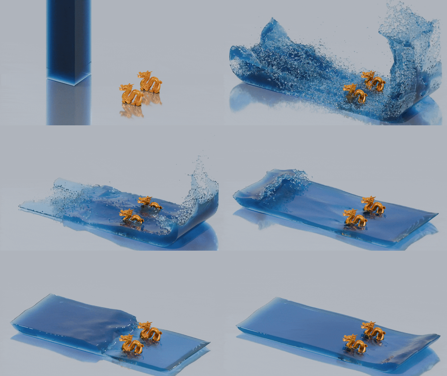
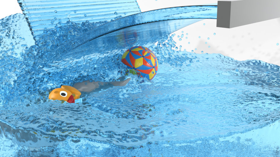
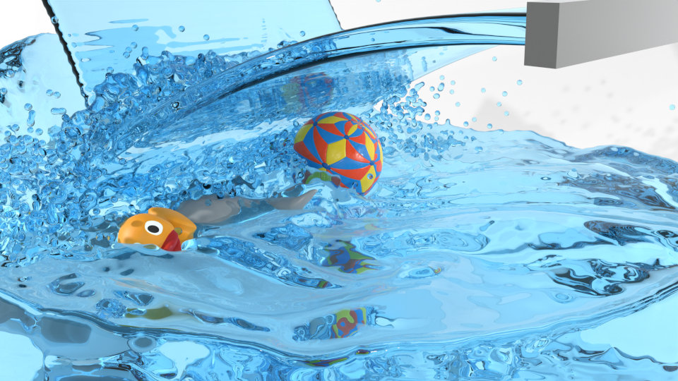
The result might look something like this:
Note: This animation does not show the recently added smoothing features of the tool, for more recent rendering see this video.
Contents
- The
splashsurfCLI - License
The following sections mainly focus on the CLI of splashsurf. For more information on the library, see the corresponding readme in the splashsurf_lib subfolder or the splashsurf_lib crate on crates.io.
The splashsurf CLI provides a "fast" marching cubes based surface reconstruction for particle data from SPH fluid simulations (e.g., performed with SPlisHSPlasH).
The output of this tool is a (closed) triangle mesh of the fluid's surface.
At the moment, it supports computing normals on the surface using SPH gradients and interpolating scalar and vector attributes defined on the particles to the surface.
To get rid of the typical bumps from SPH simulations, it supports a weighted Laplacian smoothing approach detailed below.
As input, it supports reading particle positions from .vtk/.vtu, .bgeo, .ply, .json and binary .xyz (i.e., files containing a binary dump of a particle position array) files.
Required parameters to perform a reconstruction are the kernel radius (its compact support) and particle radius (to compute the volume of particles) used for the original SPH simulation as well as the marching cubes resolution (a default iso-surface threshold is pre-configured).
A naive dense marching cubes reconstruction allocating a full 3D array over the entire fluid domain quickly becomes infeasible for larger simulations.
Instead, one could use a global hashmap where only cubes that contain non-zero fluid density values are allocated.
This approach is used in splashsurf if domain decomposition is disabled completely.
However, a global hashmap does not lead to good cache locality and is not well suited for parallelization (even specialized parallel map implementations like dashmap have their performance limitations).
To improve on this situation splashsurf utilizes a domain decomposition approach.
Since version 0.10.0, splashsurf implements a domain decomposition approach called the "subdomain grid" approach, toggled with the --subdomain-grid=on flag (default since version 0.11.0).
Here, the goal is to divide the fluid domain into subdomains with a fixed number of marching cubes cells, by default 64x64x64 cubes.
For each subdomain, a dense 3D array is allocated for the marching cubes cells.
Of course, only subdomains that contain any fluid particles are actually allocated.
For subdomains that contain only a tiny number of fluid particles (less than 5% of the largest subdomain), a hashmap is used instead to not waste too much storage.
As most domains are dense, however, the marching cubes triangulation per subdomain is very fast as it can make full use of cache locality.
The triangulation per subdomain can be performed in parallel.
To stitch the resulting meshes together, we ensure that we perform floating point operations in the same order at the subdomain boundaries, thus guaranteeing identical values (this is possible without additional synchronization).
If the field values on the subdomain boundaries are identical from both sides, the marching cubes triangulations will be topologically compatible and can be merged in a post-processing step that can also run in parallel.
Overall, this approach should almost always be faster than the octree-based approach used before version 0.10.0.
For small numbers of fluid particles (i.e., in the low thousands or less) the domain decomposition may have worse performance due to the task-based parallelism and the additional overhead of domain decomposition and stitching. In this case, you can try to disable the domain decomposition. The reconstruction will then use a global approach parallelized using thread-local hashmaps. For larger quantities of particles, the decomposition approach is always expected to be faster.
Due to the use of hash maps and multi-threading (if enabled), the output of this implementation is not deterministic.
As shown below, the tool can handle the output of large simulations. However, it was not tested with a wide range of parameters and may not be totally robust against corner-cases or extreme parameters. If you experience problems, please report them together with your input data.
The command-line tool can be built from this repository but is also available on crates.io.
If you have a Rust toolchain installed you can install splashsurf with the command
cargo install splashsurfAlternatively you can install the Python bindings using pip:
pip install pysplashsurf
Please see the README of the Python bindings for more details.
"Good" settings for the surface reconstruction depend on the original simulation and can be influenced by different conventions of different simulators. The following parameters appear to work well with simulations performed with SPlisHSPlasH. A typical set of parameters for the reconstruction is:
particle-radius: the actual radius of the fluid particles in the simulationsmoothing-length: the smoothing length used for the SPH kernel, usually set to2.0times the particle radius (this will use a cubic kernel with a compact support radius of4.0times the particle radius)surface-threshold: typically a value between0.6and0.7works wellcube-size: usually should not be chosen larger than1.0to avoid artifacts (e.g., single particles reconstructed a rhomboids), start with a value in the range of0.75to0.5and decrease/increase it if the result is too coarse or the reconstruction takes too long.
Without further post-processing, these parameters usually lead to quite "bumpy" surfaces. To obtain smoother surfaces, the parameters can be adjusted as follows:
particle-radius: can be chosen a bit larger than the particle radius of the actual simulation. A radius around 1.4 to 1.6 times larger than the original SPH particle radius seems appropriate.smoothing-length: can be set around1.2. Larger values smooth out the surface more but also artificially increase the fluid volume.surface-threshold: a good value depends on the selectedparticle-radiusandsmoothing-lengthand can be used to counteract a fluid volume increase e.g., due to a larger particle radius. In combination with the other recommended values a threshold of0.6seemed to work well.
However, a much more effective way is to perform surface smoothing as described below.
The CLI implements the paper "Weighted Laplacian Smoothing for Surface Reconstruction of Particle-based Fluids" (Löschner, Böttcher, Jeske, Bender; 2023) which proposes a fast smoothing approach to avoid typical bumpy surfaces while preventing loss of volume that typically occurs with simple smoothing methods. The following images show a rendering of a typical surface reconstruction (on the right) with visible bumps due to the particles compared to the same surface reconstruction with weighted smoothing applied (on the left):
You can see this rendering in motion in this video. To apply this smoothing, we recommend the following settings:
--mesh-smoothing-weights=on: This enables the use of special weights during the smoothing process which preserve fluid details. For more information, we refer to the paper.--mesh-smoothing-iters=25: This enables smoothing of the output mesh. The individual iterations are relatively fast, and 25 iterations appeared to strike a good balance between an initially bumpy surface and potential over-smoothing.--mesh-cleanup=on/--decimate-barnacles=on: One of the options should be used when applying smoothing, otherwise artifacts can appear on the surface (for more details see the paper). Themesh-cleanupflag enables a general purpose marching cubes mesh cleanup procedure that removes small sliver triangles everywhere on the mesh. Thedecimate-barnaclesenables a more targeted decimation that only removes specific triangle configurations that are problematic for the smoothing. The former approach results in a "nicer" mesh overall but can be slower than the latter.--normals-smoothing-iters=10: If normals are being exported (with--normals=on), this results in an even smoother appearance during rendering.
For the reconstruction parameters in conjunction with the weighted smoothing, we recommend parameters close to the simulation parameters.
That means selecting the same particle radius as in the simulation, a corresponding smoothing length (e.g., for SPlisHSPlasH a value of 2.0), a surface-threshold between 0.6 and 0.7 and a cube size usually between 0.5 and 1.0.
A full invocation of the tool might look like this:
splashsurf reconstruct particles.vtk -r=0.025 -l=2.0 -c=0.5 -t=0.6 --mesh-smoothing-weights=on --mesh-smoothing-iters=15 --normals=on --normals-smoothing-iters=10
For example:
splashsurf reconstruct canyon_13353401_particles.xyz -r=0.011 -c=1.5 -l=2.0 -t=0.6
With these parameters, a scene with 13353401 particles is reconstructed in less than 3 seconds on an Apple M4 Pro (14 cores). The output is a mesh with 6069264 triangles.
[17:34:31.034][INFO] target/release/splashsurf v0.14.0 (splashsurf)
[17:34:31.034][INFO] Called with command line: target/release/splashsurf reconstruct /Users/floeschner/Downloads/canyon_13353401_particles.xyz -r=0.011 -c=1.5 -l=2.0 -t=0.6 --output-dir=out
[17:34:31.034][INFO] Using single precision (f32) for surface reconstruction.
[17:34:31.034][INFO] Reading particle dataset from "/Users/floeschner/Downloads/canyon_13353401_particles.xyz"...
[17:34:31.093][INFO] Successfully read dataset with 13353401 particle positions.
[17:34:31.093][INFO] Vectorization enabled with support detected for NEON instructions.
[17:34:31.098][INFO] Bounding box of particles with margin for levelset evaluation: [-25.006098, -5.014629, -40.06346] to [24.499493, 18.30621, 39.775795]
[17:34:31.098][INFO] The ghost margin volume per subdomain is 42.38% of the subdomain volume
[17:34:31.098][INFO] The ghost margin per subdomain is 3.03 MC cells or 0.05 subdomains wide
[17:34:31.098][INFO] Number of subdomains: 82156 (47x23x76)
[17:34:31.098][INFO] Number of MC cells per subdomain: 262144 (64x64x64)
[17:34:31.098][INFO] Number of MC cells globally: 21536702464 (3008x1472x4864)
[17:34:31.098][INFO] Starting classification of particles into subdomains.
[17:34:31.180][INFO] Starting computation of global density vector.
[17:34:32.645][INFO] Largest subdomain has 167861 particles.
[17:34:32.645][INFO] Subdomains with 8393 or less particles will be considered sparse.
[17:34:32.645][INFO] Starting reconstruction (level-set evaluation and local triangulation).
[17:34:33.259][INFO] Starting stitching of subdomain meshes to global mesh.
[17:34:33.316][INFO] Global mesh has 3037970 vertices and 6069264 triangles.
[17:34:33.400][INFO] Writing mesh with 3037970 vertices and 6069264 cells to "out/canyon_13353401_particles_surface.vtk"...
[17:34:33.494][INFO] Successfully wrote mesh to file.
[17:34:33.501][INFO] Successfully finished processing all inputs.
[17:34:33.501][INFO] Timings:
[17:34:33.501][INFO] reconstruct subcommand: 100.00%, 2467.24ms avg, 1 call (total: 2.467s)
[17:34:33.501][INFO]   surface reconstruction: 99.99%, 2467.07ms avg, 1 call (total: 2.467s)
[17:34:33.501][INFO]     loading particle positions: 2.37%, 58.58ms avg, 1 call (total: 0.059s)
[17:34:33.501][INFO]     compute minimum enclosing aabb: 0.23%, 5.62ms avg, 1 call (total: 0.006s)
[17:34:33.501][INFO]     surface reconstruction subdomain-grid: 93.31%, 2301.96ms avg, 1 call (total: 2.302s)
[17:34:33.501][INFO]       decomposition: 3.53%, 81.29ms avg, 1 call (total: 0.081s)
[17:34:33.501][INFO]         classifying particles: 32.92%, 26.76ms avg, 1 call (total: 0.027s)
[17:34:33.501][INFO]         merging TL per cell particle counters: 0.17%, 0.14ms avg, 1 call (total: 0.000s)
[17:34:33.501][INFO]         initializing flat subdomain data and index mapping: 0.07%, 0.06ms avg, 1 call (total: 0.000s)
[17:34:33.501][INFO]         copying particles to subdomains: 52.60%, 42.76ms avg, 1 call (total: 0.043s)
[17:34:33.501][INFO]         sort subdomain particles: 14.17%, 11.52ms avg, 1 call (total: 0.012s)
[17:34:33.501][INFO]       compute_global_density_vector: 63.66%, 1465.39ms avg, 1 call (total: 1.465s)
[17:34:33.501][INFO]         subdomain density computation: ≈100.00%, 15.09ms avg, 1275 calls (total: 19.238s)
[17:34:33.501][INFO]           collect subdomain data: 0.57%, 0.09ms avg, 1275 calls (total: 0.110s)
[17:34:33.501][INFO]           initialize particle filter: 0.10%, 0.02ms avg, 1275 calls (total: 0.019s)
[17:34:33.501][INFO]           neighborhood_search_spatial_hashing_flat_filtered: 85.88%, 12.96ms avg, 1275 calls (total: 16.522s)
[17:34:33.501][INFO]             sequential_generate_cell_to_particle_map_with_positions: 5.29%, 0.69ms avg, 1275 calls (total: 0.875s)
[17:34:33.501][INFO]             collect particle neighbors: 92.97%, 12.05ms avg, 1275 calls (total: 15.360s)
[17:34:33.501][INFO]           sequential_compute_particle_densities_filtered: 12.91%, 1.95ms avg, 1275 calls (total: 2.484s)
[17:34:33.501][INFO]           update global density values: 0.53%, 0.08ms avg, 1275 calls (total: 0.102s)
[17:34:33.501][INFO]       reconstruction: 26.66%, 613.62ms avg, 1 call (total: 0.614s)
[17:34:33.501][INFO]         subdomain reconstruction (dense): ≈86.17%, 22.84ms avg, 313 calls (total: 7.148s)
[17:34:33.501][INFO]           density grid loop (neon): 79.79%, 18.22ms avg, 313 calls (total: 5.704s)
[17:34:33.501][INFO]           mc triangulation loop: 19.68%, 4.49ms avg, 313 calls (total: 1.407s)
[17:34:33.501][INFO]         subdomain reconstruction (sparse): ≈13.83%, 1.19ms avg, 962 calls (total: 1.147s)
[17:34:33.501][INFO]           density grid loop (sparse): 52.93%, 0.63ms avg, 962 calls (total: 0.607s)
[17:34:33.501][INFO]           mc triangulation loop: 46.21%, 0.55ms avg, 962 calls (total: 0.530s)
[17:34:33.501][INFO]       stitching: 2.00%, 46.06ms avg, 1 call (total: 0.046s)
[17:34:33.501][INFO]         surface patch offset scan: 0.04%, 0.02ms avg, 1 call (total: 0.000s)
[17:34:33.501][INFO]         copy interior verts/tris and deduplicate exterior verts: 82.90%, 38.18ms avg, 1 call (total: 0.038s)
[17:34:33.501][INFO]     postprocessing: 0.00%, 0.02ms avg, 1 call (total: 0.000s)
[17:34:33.501][INFO]     write surface mesh to file: 3.82%, 94.24ms avg, 1 call (total: 0.094s)
[17:34:33.501][INFO]       write_vtk: 99.90%, 94.15ms avg, 1 call (total: 0.094s)
You can either process a single file or let the tool automatically process a sequence of files.
A sequence of files is indicated by specifying a filename with a {} placeholder pattern in the name.
The tool will treat the placeholder as a (\d+) regex, i.e., a group matching to at least one digit.
This allows for any zero padding as well as non-zero padded incrementing indices.
All files in the input path matching this pattern will then be processed in natural sort order (i.e., silently skipping missing files in the sequence).
Note that the tool collects all existing filenames as soon as the command is invoked and does not update the list while running.
The first and last file of a sequences that should be processed can be specified with the -s/--start-index and/or -e/--end-index arguments.
By specifying the flag --mt-files=on, several files can be processed in parallel.
If this is enabled, you should also set --mt-particles=off as enabling both will probably degrade performance.
The combination of --mt-files=on and --mt-particles=off can be faster if many files with only few particles have to be processed.
The number of threads can be influenced using the --num-threads/-n argument or the RAYON_NUM_THREADS environment variable
NOTE: Currently, some functions do not have a sequential implementation and always parallelize over the particles or the mesh/domain. This includes:
- the new "subdomain-grid" domain decomposition approach, as an alternative to the previous octree-based approach
- some post-processing functionality (interpolation of smoothing weights, interpolation of normals and other fluid attributes)
Using the --mt-particles=off argument does not affect these parts of the surface reconstruction.
For now, it is therefore recommended to not parallelize over multiple files if this functionality is used.
Legacy VTK files with the ".vtk" extension are loaded using vtkio.
The VTK file is loaded as a big endian binary file and has to contain an "Unstructured Grid" with either f32 or f64 vertex coordinates.
Any other data or attributes are ignored except for those attributes that were specified with the --interpolate-attributes command line argument.
Currently supported attribute data types are scalar integers, floats, and three-component float vectors.
Only the first "Unstructured Grid" is loaded, other entities are ignored.
Not that currently only the "pure" v4.2 legacy format is supported as documented on here.
This corresponds to the --output-format vtk42 flag of the meshio convert tool.
VTK XML files with the ".vtu" extension are loaded using vtkio.
Currently only VTU files using ASCII or encoded binary are supported.
Files using "raw" binary sections (i.e., a <AppendedData encoding="raw">...</AppendedData> block) are not supported by vtkio at the moment.
Files with the ".bgeo" extension are loaded using a custom parser.
Note, that only the "old" BGEOV format is supported (which is the format supported by "Partio").
Both uncompressed and (gzip) compressed files are supported.
Only points and their implicit position vector attributes are loaded from the file.
All other entities (e.g., vertices) and other attributes are ignored/discarded.
Notably, the parser supports BGEO files written by SPlisHSPlasH ("Partio export").
Files with the ".ply" extension are loaded using ply-rs.
The PLY file has to contain an element called "vertex" with the properties x, y and z of type f32/"Property::Float".
Any other properties or elements are ignored.
Files with the ".xyz" extension are interpreted as raw bytes of f32 values in native endianness of the system.
Three consecutive f32s represent a (x,y,z) coordinate triplet of a fluid particle.
Files with the ".json" extension are interpreted as serializations of a Vec<[f32; 3]> where each three component array represents a particle position.
This corresponds to a JSON file with a structure like this, for example:
[
    [1.0, 2.0, 3.0],
    [1.0, 2.0, 3.0]
]Currently, only VTK and OBJ formats are supported to store the reconstructed surface meshes. Both formats support output of normals, but only VTK supports additional fields such as interpolated scalar or vector fields. The file format is inferred from the extension of output filename.
splashsurf-reconstruct (v0.14.0) - Reconstruct a surface from particle data

Usage: splashsurf reconstruct [OPTIONS] --particle-radius <PARTICLE_RADIUS> --smoothing-length <SMOOTHING_LENGTH> --cube-size <CUBE_SIZE> <INPUT_FILE_OR_SEQUENCE>

Options:
  -q, --quiet    Enable quiet mode (no output except for severe panic messages), overrides verbosity level
  -v...          Print more verbose output, use multiple "v"s for even more verbose output (-v, -vv)
  -h, --help     Print help
  -V, --version  Print version

Input/output:
  -o, --output-file <OUTPUT_FILE>  Filename for writing the reconstructed surface to disk (supported formats: VTK, PLY, OBJ, default: "{original_filename}_surface.vtk")
      --output-dir <OUTPUT_DIR>    Optional base directory for all output files (default: current working directory)
  -s, --start-index <START_INDEX>  Index of the first input file to process when processing a sequence of files (default: lowest index of the sequence)
  -e, --end-index <END_INDEX>      Index of the last input file to process when processing a sequence of files (default: highest index of the sequence)
  <INPUT_FILE_OR_SEQUENCE>         Path to the input file where the particle positions are stored (supported formats: VTK 4.2, VTU, binary f32 XYZ, PLY, BGEO), use "{}" in the filename to indicate a placeholder for a sequence

Numerical reconstruction parameters:
  -r, --particle-radius <PARTICLE_RADIUS>
          The particle radius of the input data
      --rest-density <REST_DENSITY>
          The rest density of the fluid [default: 1000.0]
  -l, --smoothing-length <SMOOTHING_LENGTH>
          The smoothing length radius used for the SPH kernel, the kernel compact support radius will be twice the smoothing length (in multiples of the particle radius)
  -c, --cube-size <CUBE_SIZE>
          The cube edge length used for marching cubes in multiples of the particle radius, corresponds to the cell size of the implicit background grid
  -t, --surface-threshold <SURFACE_THRESHOLD>
          The iso-surface threshold used for the marching cubes algorithm, this is the value of the implicit surface function (here the color field) at which the surface is reconstructed [default: 0.6]
      --particle-aabb-min <X_MIN> <Y_MIN> <Z_MIN>
          Lower corner of the domain where surface reconstruction should be performed (requires domain-max to be specified)
      --particle-aabb-max <X_MIN> <Y_MIN> <Z_MIN>
          Upper corner of the domain where surface reconstruction should be performed (requires domain-min to be specified)

Advanced parameters:
  -d, --double-precision=<off|on>  Enable the use of double precision for all computations [default: off] [possible values: off, on]
      --mt-files=<off|on>          Enable multithreading to process multiple input files in parallel (NOTE: Currently, the subdomain-grid domain decomposition approach and some post-processing functions including interpolation do not have sequential versions and therefore do not work well with this option enabled) [default: off] [possible values: off, on]
      --mt-particles=<off|on>      Enable multithreading for a single input file by processing chunks of particles in parallel [default: on] [possible values: off, on]
  -n, --num-threads <NUM_THREADS>  Set the number of threads for the worker thread pool
      --simd=<off|on>              Enable vectorization of some computations using SIMD instructions (requires CPU with AVX2 or NEON support). Note that vectorization is currently only available in single precision (f32) mode [default: on] [possible values: off, on]

Domain decomposition parameters:
      --subdomain-grid=<off|on>
          Enable automatic spatial decomposition using a regular grid-based approach (for efficient multithreading) if the domain is large enough [default: on] [possible values: off, on]
      --subdomain-grid-auto-disable=<off|on>
          Whether to automatically disable the spatial decomposition if the domain is too small [default: on] [possible values: off, on]
      --subdomain-cubes <SUBDOMAIN_CUBES>
          Each subdomain will be a cube consisting of this number of MC grid cells along each coordinate axis [default: 64]

Interpolation & normals:
      --normals=<off|on>
          Enable computing surface normals at the mesh vertices and write them to the output file [default: off] [possible values: off, on]
      --sph-normals=<off|on>
          Enable computing the normals using SPH interpolation instead of using the area weighted triangle normals [default: off] [possible values: off, on]
      --normals-smoothing-iters <NORMALS_SMOOTHING_ITERS>
          Number of smoothing iterations to apply to normals if normal interpolation is enabled (disabled by default)
      --output-raw-normals=<off|on>
          Enable writing raw normals without smoothing to the output mesh if normal smoothing is enabled [default: off] [possible values: off, on]
  -a, --interpolate_attribute <ATTRIBUTE_NAME>
          Interpolate a point attribute field with the given name from the input file to the reconstructed surface. Currently, this is only supported for BGEO, VTK and VTU input files. Specify the argument multiple times for each attribute that should be interpolated

Mesh decimation and cleanup:
      --mesh-cleanup=<off|on>
          Enable MC specific mesh decimation/simplification which removes bad quality triangles typically generated by MC by snapping (enabled by default if smoothing is enabled) [default: off] [possible values: off, on]
      --mesh-cleanup-snap-dist <MESH_CLEANUP_SNAP_DIST>
          If MC mesh cleanup is enabled, vertex snapping can be limited to this distance relative to the MC edge length (should be in range of [0.0,0.5])
      --decimate-barnacles=<off|on>
          Enable decimation of some typical bad marching cubes triangle configurations (resulting in "barnacles" after Laplacian smoothing) [default: off] [possible values: off, on]
      --keep-verts=<off|on>
          Enable preserving vertices without connectivity during decimation instead of filtering them out (faster and helps with debugging) [default: off] [possible values: off, on]

Mesh smoothing:
      --mesh-smoothing-iters <MESH_SMOOTHING_ITERS>
          Number of smoothing iterations to run on the reconstructed mesh
      --mesh-smoothing-weights=<off|on>
          Enable feature weights for mesh smoothing if mesh smoothing enabled. Preserves isolated particles even under strong smoothing [default: off] [possible values: off, on]
      --mesh-smoothing-weights-normalization <MESH_SMOOTHING_WEIGHTS_NORMALIZATION>
          Override a manual normalization value from weighted number of neighbors to mesh smoothing weights [default: 13.0]
      --output-smoothing-weights=<off|on>
          Enable writing the smoothing weights as a vertex attribute to the output mesh file [default: off] [possible values: off, on]

General postprocessing:
      --generate-quads=<off|on>
          Enable conversion of triangles to quads if they meet quality criteria [default: off] [possible values: off, on]
      --quad-max-edge-diag-ratio <QUAD_MAX_EDGE_DIAG_RATIO>
          Maximum allowed ratio of quad edge lengths to its diagonals to merge two triangles to a quad (inverse is used for minimum) [default: 1.75]
      --quad-max-normal-angle <QUAD_MAX_NORMAL_ANGLE>
          Maximum allowed angle (in degrees) between triangle normals to merge them to a quad [default: 10]
      --quad-max-interior-angle <QUAD_MAX_INTERIOR_ANGLE>
          Maximum allowed vertex interior angle (in degrees) inside a quad to merge two triangles to a quad [default: 135]
      --mesh-aabb-min <X_MIN> <Y_MIN> <Z_MIN>
          Lower corner of the bounding-box for the surface mesh, triangles completely outside are removed (requires mesh-aabb-max to be specified)
      --mesh-aabb-max <X_MIN> <Y_MIN> <Z_MIN>
          Upper corner of the bounding-box for the surface mesh, triangles completely outside are removed (requires mesh-aabb-min to be specified)
      --mesh-aabb-clamp-verts=<off|on>
          Enable clamping of vertices outside the specified mesh AABB to the AABB (only has an effect if mesh-aabb-min/max are specified) [default: off] [possible values: off, on]
      --output-raw-mesh=<off|on>
          Enable writing the raw reconstructed mesh before applying any post-processing steps (like smoothing or decimation) [default: off] [possible values: off, on]

Debug options:
      --check-mesh=<off|on>
          Enable checking the final mesh for holes and non-manifold edges and vertices [default: off] [possible values: off, on]
      --check-mesh-closed=<off|on>
          Enable checking the final mesh for holes [default: off] [possible values: off, on]
      --check-mesh-manifold=<off|on>
          Enable checking the final mesh for non-manifold edges and vertices [default: off] [possible values: off, on]
      --check-mesh-orientation=<off|on>
          Enable checking the final mesh for inverted triangles (compares angle between vertex normals and adjacent face normals) [default: off] [possible values: off, on]
      --check-mesh-debug=<off|on>
          Enable additional debug output for the check-mesh operations (has no effect if no other check-mesh option is enabled) [default: off] [possible values: off, on]
Allows conversion between particle file formats and between mesh file formats. For particles VTK, BGEO, PLY, XYZ, JSON -> VTK
is supported. For meshes only VTK, PLY -> VTK, OBJ is supported.
splashsurf-convert (v0.13.0) - Convert particle or mesh files between different file formats

Usage: splashsurf convert [OPTIONS] -o <OUTPUT_FILE>

Options:
      --particles <INPUT_PARTICLES>
          Path to the input file with particles to read (supported formats: .vtk, .vtu, .bgeo, .ply, .xyz, .json)
  -q, --quiet
          Enable quiet mode (no output except for severe panic messages), overrides verbosity level
      --mesh <INPUT_MESH>
          Path to the input file with a surface to read (supported formats: .vtk, .ply)
  -v...
          Print more verbose output, use multiple "v"s for even more verbose output (-v, -vv)
  -o <OUTPUT_FILE>
          Path to the output file (supported formats for particles: .vtk, .bgeo, .json, for meshes: .obj, .vtk)
      --overwrite
          Whether to overwrite existing files without asking
      --domain-min <X_MIN> <Y_MIN> <Z_MIN>
          Lower corner of the domain of particles to keep (requires domain-max to be specified)
      --domain-max <X_MIN> <Y_MIN> <Z_MIN>
          Lower corner of the domain of particles to keep (requires domain-min to be specified)
  -h, --help
          Print help
  -V, --version
          Print version
To cite splashsurf you can use this BibTeX entry:
@inproceedings {LBJB23,
  booktitle = {Vision, Modeling, and Visualization},
  title = {{Weighted Laplacian Smoothing for Surface Reconstruction of Particle-based Fluids}},
  author = {Löschner, Fabian and Böttcher, Timna and Rhys Jeske, Stefan and Bender, Jan},
  year = {2023},
  publisher = {The Eurographics Association},
  DOI = {10.2312/vmv.20231245}
}This project contains notable contributions from the following people:
- Timna Böttcher (@timnaboettcher): co-developed the weighted smoothing approach
- Felix Kern (@Fek04): implemented the Python bindings for
splashsurf - Fabian Löschner (@w1th0utnam3): implemented most of the surface reconstruction library and CLI with the domain decomposition
For license information of this project, see the LICENSE file. The splashsurf logo is based on two graphics (1, 2) published on SVG Repo under a CC0 ("No Rights Reserved") license. The dragon model shown in the images on this page is part of the "Stanford 3D Scanning Repository".


