Vehicle State Estimation on a Roadway

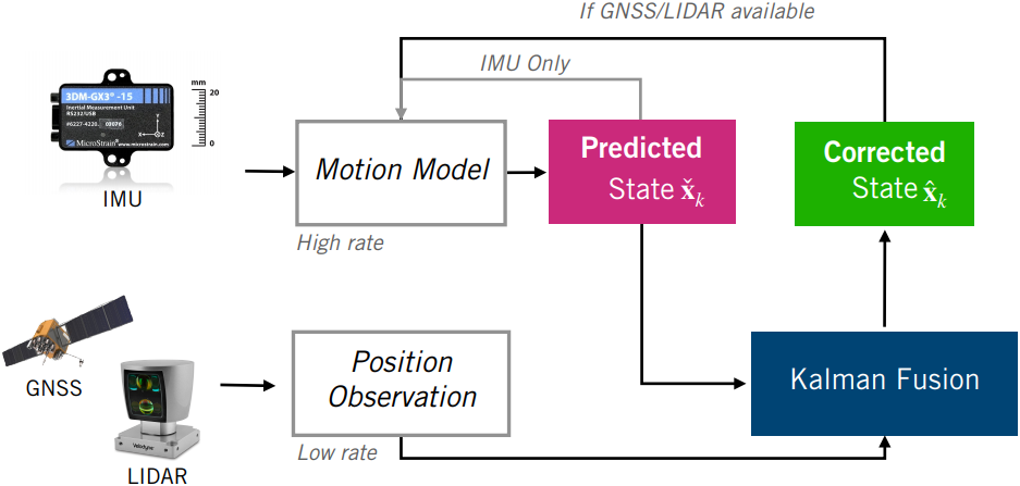
This project implements the Error-State Extended Kalman Filter (ES-EKF) to localize a vehicle using data from the CARLA simulator. The following diagram shows a graphical representation of the system.

This project is the final programming assignment of the State Estimation and Localization for Self-Driving Cars course from Coursera. The starter code is provided by the University of Toronto.

The Kalman Filter algorithm updates a state estimate through two stages:

prediction using the motion model
correction using the measurement model

1. Preliminaries
- 1.1. Vehicle State Initialization
2. Prediction
3. Correction
4. Vehicle Trajectory
- 4.1. Ground Truth and Estimate
- 4.2. Estimation Error and Uncertainty Bounds

1. Preliminaries

1.1. Vehicle State Initialization

The vehicle state at each time step consists of position, velocity, and orientation (parameterized by a unit quaternion); the inputs to the motion model are the IMU specific force and angular rate measurements.

Description	Equation
Vehicle State	$\boldsymbol{\x}_k=[\boldsymbol{\p}_k, \boldsymbol{\v}_k, \boldsymbol{\q}_k]^{T} \in R^10$
IMU Measurements	$\boldsymbol{\u}_k=[\boldsymbol{\f}_k, \boldsymbol{\omega}_k]^{T} \in R^6$

This section of code initializes the variables for the ES-EKF solver.

p_est = np.zeros([imu_f.data.shape[0], 3])  # position estimates
v_est = np.zeros([imu_f.data.shape[0], 3])  # velocity estimates
q_est = np.zeros([imu_f.data.shape[0], 4])  # orientation estimates as quaternions
p_cov = np.zeros([imu_f.data.shape[0], 9, 9])  # covariance matrices at each timestep

# Set initial values.
p_est[0] = gt.p[0]
v_est[0] = gt.v[0]
q_est[0] = Quaternion(euler=gt.r[0]).to_numpy()
p_cov[0] = np.zeros(9)  # covariance of estimate
gnss_i  = 0
lidar_i = 0

2. Prediction

The main filter loop operates by first predicting the next state (vehicle pose and velocity). The predicted vehicle state integrates the high-rate IMU measurements by using a nonlinear motion model.

2.1. Motion Model

The motion model of the vehicle is given by the following set of equations

Description	Equation
Position	$\boldsymbol{\p}_k = \boldsymbol{\p}_{k-1} + {\Delta}t\boldsymbol{\v}_{k-1} + \frac{{\Delta}t^2}{2}(\boldsymbol{\C}_{ns}\boldsymbol{\f}_{k-1} + \boldsymbol{\g})$
Velocity	$\boldsymbol{\v}_{k} = \boldsymbol{\v}_{k-1} + {\Delta}t(\boldsymbol{\C}_{ns}\boldsymbol{\f}_{k-1} + \boldsymbol{\g})$
Orientation	$\boldsymbol{\q}_{k}=\boldsymbol{\q}_{k-1}\otimes\boldsymbol{\q}(\boldsymbol{\omega}_{k-1}{\Delta}t)=\boldsymbol{\Omega}(\boldsymbol{\q}(\boldsymbol{\omega}_{k-1}{\Delta}t))\boldsymbol{\q}_{k-1}$

2.2. Predicted State

The predicted vehicle state is therefore given by the equations

Description	Equation	Variable
Predicted State	$\boldsymbol{\check{\x}}_{k}=[\boldsymbol{\check{\p}}_{k}, \boldsymbol{\check{\v}}_{k}, \boldsymbol{\check{\q}}_{k}]^T$	`x_check`
Predicted Position	$\boldsymbol{\check{\p}}_k = \boldsymbol{\p}_{k-1} + {\Delta}t\boldsymbol{\v}_{k-1} + \frac{{\Delta}t^2}{2}(\boldsymbol{\C}_{ns}\boldsymbol{\f}_{k-1} + \boldsymbol{\g})$	`p_check`
Predicted Velocity	$\boldsymbol{\check{\v}}_{k} = \boldsymbol{\v}_{k-1} + {\Delta}t(\boldsymbol{\C}_{ns}\boldsymbol{\f}_{k-1} + \boldsymbol{\g})$	`v_check`
Predicted Orientation	$\boldsymbol{\check{\q}}_{k}=\boldsymbol{\q}_{k-1}\otimes\boldsymbol{\q}(\boldsymbol{\omega}_{k-1}{\Delta}t)$	`q_check`

This section of code iterates through the IMU inputs and updates the state.

for k in range(1, imu_f.data.shape[0]):  # start at 1 b/c we have initial prediction from gt
    delta_t = imu_f.t[k] - imu_f.t[k - 1]

    # 1. Update state with IMU inputs
    q_prev = Quaternion(*q_est[k - 1, :]) # previous orientation as a quaternion object
    q_curr = Quaternion(axis_angle=(imu_w.data[k - 1]*delta_t)) # current IMU orientation
    c_ns = q_prev.to_mat() # previous orientation as a matrix
    f_ns = (c_ns @ imu_f.data[k - 1]) + g # calculate sum of forces
    p_check = p_est[k - 1, :] + delta_t*v_est[k - 1, :] + 0.5*(delta_t**2)*f_ns
    v_check = v_est[k - 1, :] + delta_t*f_ns
    q_check = q_prev.quat_mult_left(q_curr)

2.3. Error State Linearization

In the previous section, we propagated the nominal state (x_check) forward in time. However, this prediction ignores noise and perturbations. The ES-EKF algorithm captures these deviations in the error state vector.

The next step is to consider the linearized error dynamics of the system.

Description	Equation
Error State	$\delta\boldsymbol{\x}_{k}=[\delta\boldsymbol{\p}_{k}, \delta\boldsymbol{\v}_{k}, \delta\boldsymbol{\phi}_{k}]^T \in R^9$
Error Dynamics	$\delta\boldsymbol{\x}_{k}=\boldsymbol{\F}_{k-1}\delta\boldsymbol{\x}_{k-1}+\boldsymbol{\L}_{k-1}\boldsymbol{\n}_{k-1}$
Measurement Noise	$\boldsymbol{\n}_{k}\sim N(\boldsymbol{0}, \boldsymbol{Q}_{k})$

The Jacobians and the noise covariance matrix are defined as follows

Description	Equation	Variable
Motion Model Jacobian	$\boldsymbol{\F}_{k-1}=\begin{bmatrix}\boldsymbol{\I}&\boldsymbol{\I}\cdot\Delta t&0\\0&\boldsymbol{\I}&-[\boldsymbol{\C}_{ns}\boldsymbol{\f}_{k-1}]_{\times}\Delta t\\0&0&\boldsymbol{\I}\end{bmatrix}$	`f_jac`
Motion Model Noise Jacobian	$\boldsymbol{\L}_{k-1}=\begin{bmatrix}0&0\\\boldsymbol{\I}&0\\0&\boldsymbol{\I}\end{bmatrix}$	`l_jac`
IMU Noise Covariance	$\boldsymbol{\Q}_{k}=\Delta t^2\begin{bmatrix}\boldsymbol{I}\cdot\sigma_{acc}^2&0\\0&\boldsymbol{I}\cdot\sigma_{gyro}^2\end{bmatrix}$	`q_cov`

where I is the 3 by 3 identity matrix.

This section of code calculates the motion model Jacobian

    # 1.1 Linearize the motion model and compute Jacobians
    f_jac = np.eye(9) # motion model jacobian with respect to last state
    f_jac[0:3, 3:6] = np.eye(3)*delta_t
    f_jac[3:6, 6:9] = -skew_symmetric(c_ns @ imu_f.data[k - 1])*delta_t

2.4. Propagate Uncertainty

In the previous section, we computed the Jacobian matrices of the motion model. We will use these matrices to propagate the state uncertainty forward in time.

The uncertainty in the state is captured by the state covariance (uncertainty) matrix. The uncertainty grows over time until a measurement arrives.

Description	Equation	Variable
Predicted State Covariance	$\boldsymbol{\check{\P}}_{k}=\boldsymbol{\F}_{k-1}\boldsymbol{\P}_{k-1}\boldsymbol{\F}_{k-1}^{T}+\boldsymbol{\L}_{k-1}\boldsymbol{\Q}_{k-1}\boldsymbol{\L}_{k-1}^{T}$	`p_cov_check`

This section of code calculates the state uncertainty

    # 2. Propagate uncertainty
    q_cov = np.zeros((6, 6)) # IMU noise covariance
    q_cov[0:3, 0:3] = delta_t**2 * np.eye(3)*var_imu_f
    q_cov[3:6, 3:6] = delta_t**2 * np.eye(3)*var_imu_w
    p_cov_check = f_jac @ p_cov[k - 1, :, :] @ f_jac.T + l_jac @ q_cov @ l_jac.T

3. Correction

3.1. Measurement Availability

The IMU data arrives at a faster rate than either GNSS or LIDAR sensor measurements.

The algorithm checks the measurement availability and calls a function to correct our prediction.

    # 3. Check availability of GNSS and LIDAR measurements
    if imu_f.t[k] in gnss_t:
        gnss_i = gnss_t.index(imu_f.t[k])
        p_check, v_check, q_check, p_cov_check = \
            measurement_update(var_gnss, p_cov_check, gnss.data[gnss_i], p_check, v_check, q_check)
    
    if imu_f.t[k] in lidar_t:
        lidar_i = lidar_t.index(imu_f.t[k])
        p_check, v_check, q_check, p_cov_check = \
            measurement_update(var_lidar, p_cov_check, lidar.data[lidar_i], p_check, v_check, q_check)

3.2. Measurement Model

The measurement model is the same for both sensors. However, they have different noise covariance.

Description	Equation
Measurement Model	$\begin{split} \boldsymbol{y}_{k} &= \boldsymbol{h}(\boldsymbol{x}_{k})+\boldsymbol{v}_{k} \\ & =\boldsymbol{H}_{k}\boldsymbol{x}_{k}+\boldsymbol{v}_{k} \\ & = \boldsymbol{p}_{k}+\boldsymbol{v}_{k} \end{split}$
GNSS Measurement Noise	$\boldsymbol{v}_{k} \sim N(0, \boldsymbol{R}_{\GNSS})$
LIDAR Measurement Noise	$\boldsymbol{v}_{k} \sim N(0, \boldsymbol{R}_{\LIDAR})$

3.3. Measurement Update

Measurements are processed sequentially by the EKF as they arrive; in our case, both the GNSS receiver and the LIDAR provide position updates.

Description	Equation	Variable
Measurement Model Jacobian	$\boldsymbol{H}_{k}=\begin{bmatrix}\boldsymbol{I}&0&0\\\end{bmatrix}$	`h_jac`
Sensor Noise Covariance	$\boldsymbol{R}=\boldsymbol{I}\cdot\sigma_{\sensor}^2$	`r_cov`
Kalman Gain	$\boldsymbol{K}_{k}=\boldsymbol{\check{P}}_{k}\boldsymbol{H}_{k}^{T}(\boldsymbol{H}_{k}\boldsymbol{\check{P}}_{k}\boldsymbol{H}_{k}^{T}+\boldsymbol{R})^{-1}$	`k_gain`

This section of code defines the measurement update function

def measurement_update(sensor_var, p_cov_check, y_k, p_check, v_check, q_check):
    # 3.1 Compute Kalman Gain
    r_cov = np.eye(3)*sensor_var
    k_gain = p_cov_check @ h_jac.T @ np.linalg.inv((h_jac @ p_cov_check @ h_jac.T) + r_cov)

We use the Kalman gain to compute the error state. Considering the innovation or difference between our predicted vehicle position, p_check, and the measured position, y_k.

Description	Equation	Variable
Error State	$\delta\boldsymbol{x}_{k}=\boldsymbol{K}_{k}(\boldsymbol{y}_{k}-\boldsymbol{\check{p}}_{k})$	`error_state`

The error state is then used to update the nominal state vector. We also calculate the corrected nominal state covariance matrix, p_cov_hat.

Description	Equation	Variable
Corrected Position	$\hat{\boldsymbol{p}}_{k}=\check{\boldsymbol{p}}_{k}+\delta\boldsymbol{p}_{k}$	`p_hat`
Corrected Velocity	$\hat{\boldsymbol{v}}_{k}=\check{\boldsymbol{v}}_{k}+\delta\boldsymbol{v}_{k}$	`v_hat`
Corrected Orientation	$\hat{\boldsymbol{q}}_{k}=\boldsymbol{q}(\delta\boldsymbol{\phi}_{k})\otimes\check{\boldsymbol{q}}_{k}$	`q_hat`
Corrected State Covariance	$\hat{\boldsymbol{P}}_{k}=(\boldsymbol{I}-\boldsymbol{K}_{k}\boldsymbol{H}_{k})\check{\boldsymbol{P}}_{k}$	`p_cov_hat`

Finally, the function returns the corrected state and state covariants.

    # 3.2 Compute error state
    error_state = k_gain @ (y_k - p_check)

    # 3.3 Correct predicted state
    p_hat = p_check + error_state[0:3]
    v_hat = v_check + error_state[3:6]
    q_hat = Quaternion(axis_angle=error_state[6:9]).quat_mult_left(Quaternion(*q_check))

    # 3.4 Compute corrected covariance
    p_cov_hat = (np.eye(9) - k_gain @ h_jac) @ p_cov_check

    return p_hat, v_hat, q_hat, p_cov_hat

4. Vehicle Trajectory

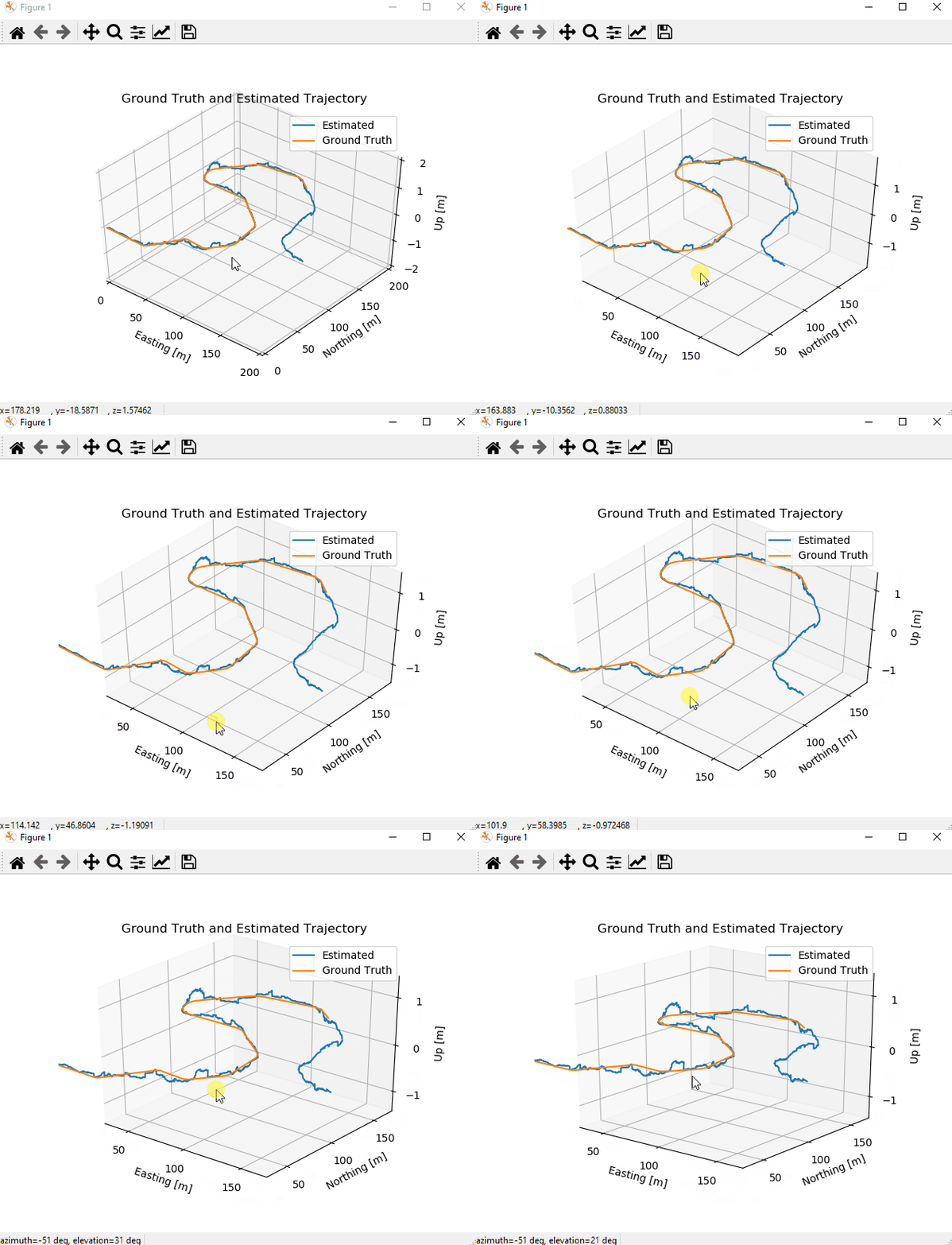
We evaluate the algorithm performance by comparing the estimated vehicle trajectory and the ground truth. The source code generates visualizations by running the following command in the terminal.

python es_ekf.py

4.1. Ground Truth and Estimate

This figure shows a comparison between the trajectory estimate and the ground truth.

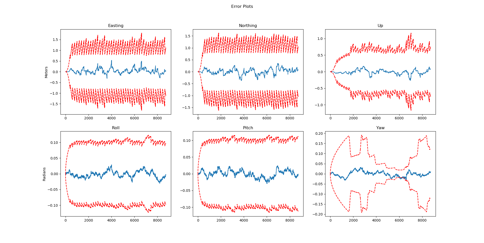
4.2. Estimation Error and Uncertainty Bounds

This figure shows our estimator error relative to the ground truth. The dashed red lines represent three standard deviations from the ground truth, according to our estimator. These lines indicate how well our model fits the actual dynamics of the vehicle and how well the estimator is performing overall. The estimation error should remain within the three-sigma bounds at all times.

Kingshida/Vehicle-State-Estimation