Author: Léo-Paul Dagallier
Last update: 2023-11-28
This repository presents the biogeographic and diversification analyses of the Monodoreae (Annonaceae family) carried out in Dagallier, Condamine & Couvreur, 2023.
Feel free to open an issue if you have any question.
If you make use of scripts published in this repository, please cite:
Dagallier L-PMJ, Condamine FL, Couvreur TLP (2023) A sequential diversification with Miocene extinction and Pliocene speciation linked to mountain uplift explains the diversity of the African rain forest clade Monodoreae (Annonaceae). Annals of Botany: mcad130. https://doi.org/10.1093/aob/mcad130
The time-calibrated phylogenetic tree of the Monodoreae was reconstructed in a Bayesian framework using BEAST and 2 fossil calibration (see details in Material & Methods).
The tree:
library(ape)
library(phylotools)
library(ggtree)
library(ggplot2)
library(treeio)
library(tidyverse)
sub_table = read.table(file = "data/sub_table.txt")
treefile = c("MCC_monodoreae3_subset32var_ucld_ch1.tree")
tree <- treeio::read.beast(paste0("data/", treefile)) # reads the MCC tree in BEAST format
tree@phylo <- sub.taxa.label(tree@phylo, sub_table) # Replace the label name
write.beast(tree, file = paste0("data/name_", treefile)) # write the tree back in nexus format
Plot the tree with annotations:
# Define a custom geological time scale (GTS)
library(deeptime)
GTS <- force(epochs)
GTS_perso <- GTS
GTS_perso$name[2] = "Ple."
GTS_perso$name[3] = "Pli."
# Load geographical data
geo <- read_tsv("data/geo_distribution_species.txt", col_names = c("label", "geo"), na = c("", "na"))
tree <- full_join(tree, geo, by = 'label')
gg = (ggtree(tree) +
# plot tree, HPD, node support, tips
geom_range(range='height_0.95_HPD', alpha=.6, size=2, color='#695eff', center = 'height') +
geom_nodelab(aes(x=x, label=round(height,2)), hjust=-.2, size=2) +
geom_point2(aes(subset=!isTip & posterior <1, fill=cut(posterior, c(0, 0.9, 1))), shape=21, size=2, stroke = 0.3)+
geom_nodelab(aes(x=x, label=round(posterior,2), subset=!isTip & posterior <1), size=0.8) +
geom_tiplab(offset = 1, size = 2.5)+
# geographical distribution
geom_point2(aes(x = x+1, subset=isTip, color= geo), shape = 15, size = 2)+
# fossils calibrations
geom_point2(aes(subset=node %in% c(120, 119)), position = position_nudge(y = 4), shape = 25, fill = "#fb6a4a", stroke = 0, size = 3)+
# annotations
annotate(geom = "text", x = -90, y = 118, label = "Annonaceae", hjust = -0.05, vjust = 1, size = 5)+
annotate(geom = "text", x = -25, y = 118, label = "Monodoreae", hjust = -0.05, vjust = 1, size = 5)+
annotate(geom = "point", x = -120, y = 70, shape = 25, fill = "#fb6a4a", stroke = 0, size = 3)+
annotate(geom = "text", x = -118, y = 70, label = "Fossil calibration point", hjust = 0)+
# geological time scale
coord_geo(neg = T, pos = "b", dat = GTS_perso, abbrv = F, height = unit(1, "line"), size = 2.7, bord = c(), skip = c( "Holocene"), center_end_labels = T, expand = T)+
# layout elements
theme_tree2() +
scale_fill_manual(values=c("grey", "white"), guide='legend',
name='Posterior Probability (PP)',
breaks=c('(0.9,1]', '(0,0.9]'),
labels=expression(0.9 <= PP * " < 1", PP < 0.9))+
scale_color_manual(values = c("centre" = "#1f78b4", "east" = "#33a02c", "mada" = "#fdbf6f","west" = "#6a3d9a"), na.value = "transparent",
name = "Geographical distribution",
labels = c("centre" = "Central Africa", "east" = "East Africa", "mada" = "Madagascar","west" = "West Africa"))+
theme(axis.line.x.bottom = element_line("#bdbdbd"),
panel.grid.major.x = element_line("#bdbdbd"),
panel.grid.minor.x = element_line("#f0f0f0"),
legend.position=c(0.1, 0.8),
legend.background = element_blank(),
legend.key = element_blank())) %>% revts()+ scale_x_continuous(labels=abs, breaks = c(0,-20, -40, -60, -80, -100, -120), limits = c(-120, 30)) + geom_highlight(node=120, fill="steelblue", alpha=.1, to.bottom = T, xmin = -90) + geom_highlight(node=126, fill="darkgreen", alpha=.2, to.bottom = T, xmin = -24.9)
# save as pdf
pdf(file = paste0("figures/", "name_MCC_monodoeae3_monod_full_Annon_GTS",".pdf"), width = 13 , height = 10)
gg
dev.off()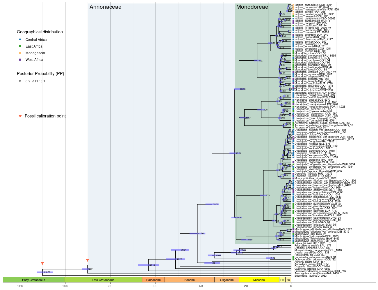 This figure can be
viewed here
The downstream analysis will be run only on the Monodoreae. We thus need to subset the Monodoreae tribe to the tree above.
Subset the Monodoreae tribe (node 126) from this dataset:
library(treeio)
tree_monod <- treeio::tree_subset(tree, node = 126, levels_back = 0)
write.tree(as.phylo(tree_monod), file = "data/name_MCC_monodoeae3_monod.newick")For the biogeographic analysis (ancestral range reconstruction), we need only one representative per species (i.e. no variety or subspecies). Remove the duplicates in the tree:
to_drop = c("Asteranthe_asterias_subsp_triangularis-DAG_10",
            "Hexalobus_monopetalus-LOT_1671",
            "Isolona_campanulata-MUN_6",
            "Mischogyne_elliotiana_var_sericea-DEI_3015",
            "Monodora_crispata-KWA_19",
            "Monodora_myristica-HAW_93",
            "Monodora_tenuifolia-BUR_1798",
            "Monodora_undulata-JON_7637_W",
            "Uvariastrum_pierreanum-JON_7190",
            "Uvariodendron_calophyllum-MER_1385",
            "Uvariodendron_fuscum_var_magnificum-HAM_676",
            "Uvariodendron_fuscum_var_fuscum-MIL_6428",
            "Uvariopsis_congensis_var_angustifolia-WHI_3334",
            "Uvariopsis_guineensis_var_globiflora-JON_1809",
            "Uvariopsis_solheidi_var_letestui-COU_550",
            "Dennettia_tripetala-HAL_43276")
tree_monod_pruned <- drop.tip(tree_monod, to_drop)
write.tree(as.phylo(tree_monod_pruned), file = "data/name_MCC_monodoreae3_monod_pruned.newick")
write.beast(tree_monod_pruned, file = "data/name_MCC_monodoreae3_monod_pruned.tree")
The details about the biogeographic analysis can be found here:
Biogeographic analyses.
Bayesian Analysis of Macroevolutionary Mixtures. All the analysis are
detailed here: BAMM.
No significant rate shift detected:
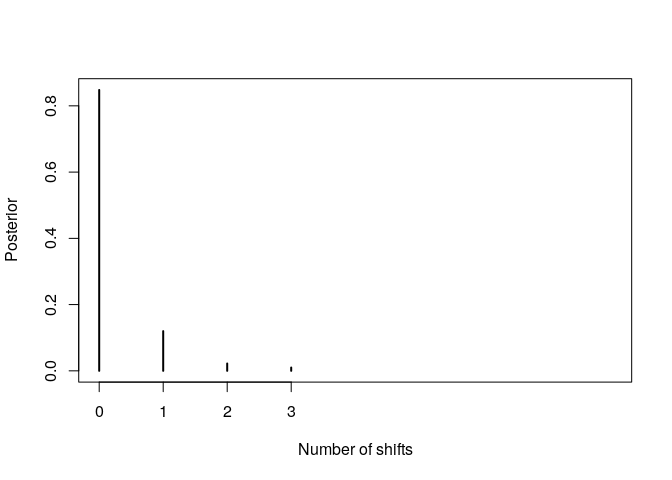
The estimated speciation rate is constant across the time. It
appears higher for Uvariopsis: 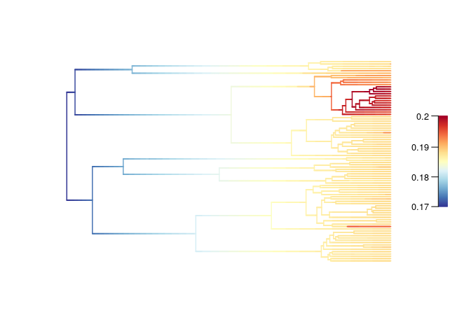
The estimated extinction rate is constant across the time:
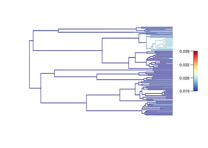
The estimated net diversification rate is constant across the time.
It appears higher for Uvariopsis: 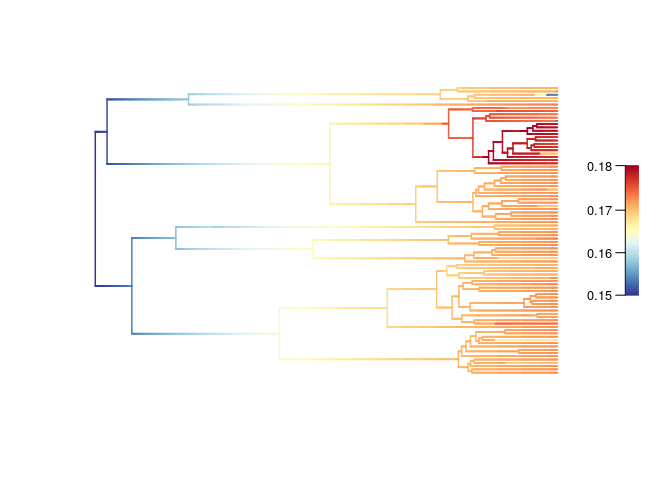
Species-specific diversification rate shifts. See: ‘Maliet et al. 2019’ & ‘Maliet & Morlon 2022’.
All the analysis detailed here: ClaDS.
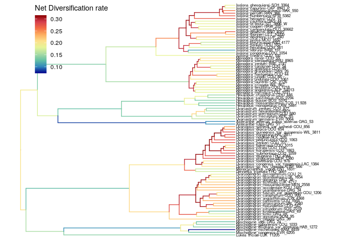
The branch specific speciation rate is the highest for the species-rich
genus Uvariopsis, and high for the other species-rich genera
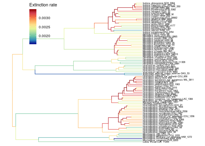
Isolona, Monodora, and Uvariodendron. 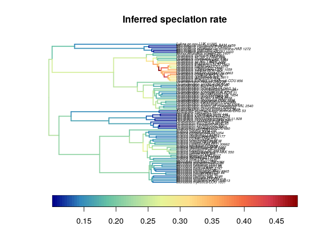 We observe a similar
pattern for the extinction rate, although the values are very low:

See RevBayes_BSDR.
With RevBayes, we find a similar result than ClaDS: speciation rate is
the highest for the species-rich genus Uvariopsis, and high for the
other species-rich genera Isolona, Monodora, and Uvariodendron.
Note that for Isolona and Monodora, the speciation rate is
particularly high at the root of the genera.
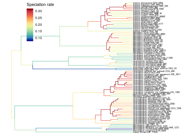
The extinction rate is very low.
The net diversification rate is similar to the speciation rate.
Results of the CoMET analysis. All the analysis detailed here:
CoMET.
With a probability of 5% to survive a mass extinction event:
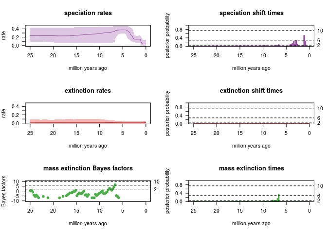
With a probability of 5% to survive a mass extinction event:
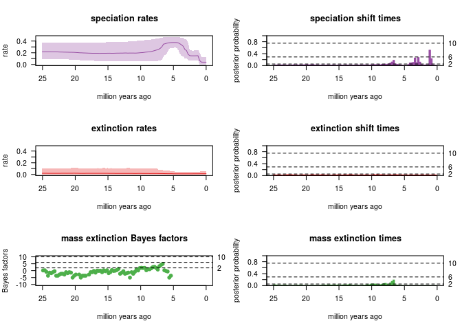
- Extinction rate is low, no rate shift detected
- Mass extinction:
- the analysis strongly detects (2lnBF>6) a ME event 6-7 My ago in case the a priori probability of survival to a ME event is 5%
- the analysis substantially detects a ME event in case the a priori probability of survival to a ME event is 30%
- Significant speciation rate shift detected ~2 My ago
Summary of all the CoMET analysis: 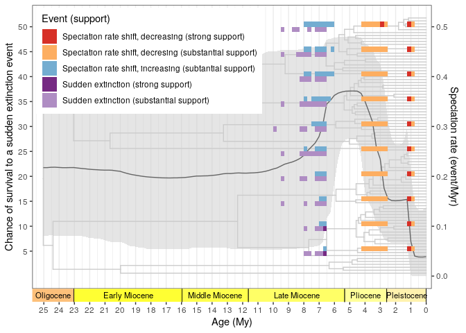 ### RPANDA
Results of the RPANDA analysis. All the analysis detailed here:
RPANDA.
The best fitting model appear to be the Pure Birth model with λ =
0.17495781 (AICc = 473.5). 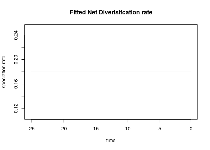
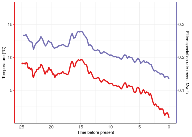
Temperature data from Condamine et al. 2015.
The best fitting model appear to be the Pure Birth model with speciation varying exponentially with temperatures: λ = 0.1255 and α = 0.0829 (AICc = 472.4, ΔAICc = 1.07).
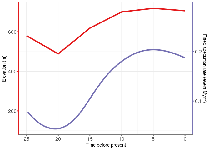
Paleo-elevation data retrieved from paleo-Digital Elevation Models
‘paleoDEMs’ from
PaleoMaps
with the chronosphere package.
First, I retrieved the convex envelop of the distribution of the Monodoreae tribe (from geo-referenced specimens). I then computed the mean elevation of the African land within this envelope. I did so for the current land elevation and for the past land elevation at times 5, 10, 15 20, 25 and 30 Myr before present. The PaleMap dataset doesn’t have the paleoDEMs between these times. The geographic precision is 1 degree and the altitude precision is 40 meters. See PaleoElevation for the details.
The best fitting model appear to be the Pure Birth model with speciation varying exponentially with elevation: λ = 0.001725 and α = 0.0066 (AICc = 469.3, ΔAICc = 2.26).
Some best fitting models retrieve extinction rates higher than speciation rates (leading to negative net diversification rates). These models are unrealistic and are discarded. See RPANDA_C4 and the main text in the article.
