Levin Jian, June 2017
PASCAL VOC is a publicly available benchmark dataset used for object recognition and detection. There are about 17k images in the dataset (VOC 2007 and VOC 2012), and contains 20 labelled classes like person, car, cat, bottle, bicycle, sheep, sofa, and etc. The detector we develooped can be used to determine what kind of objects an image contains, and where those objects are.
We used the excellent work from here as our baseline. The baseline successfully converted the original SSD detector from caffe implementation to tensorflow implementation. The goal of our project is to focus on the trainig part of the problem. Specifically, We load the VGG16 weights trained from ImageNET into our VGG 16 part of SSD model, train SSD modle on PASCAL VOC training dataset (VOC 2007 train_eval and VOC 2012 train_eval), and evaluat SSD model on PASCAL VOC test dataset (VOC 2007 test). Evaluation metric is mAP.
Techncially, tensorflow and slim are used as the neural network framework, and all the development is done in Python.
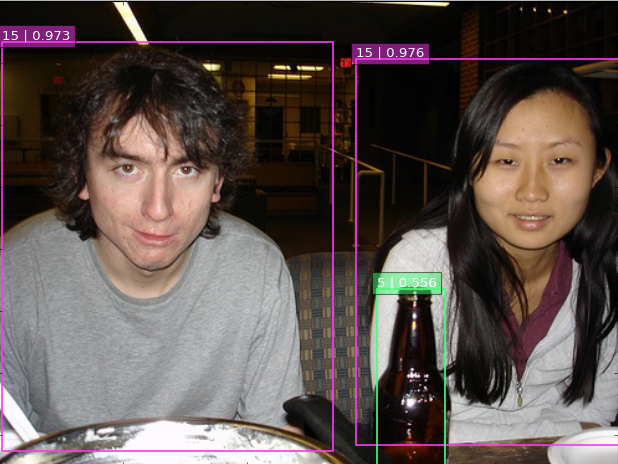
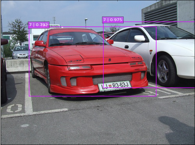
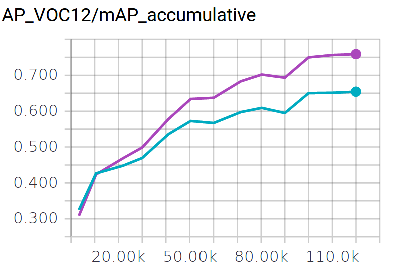
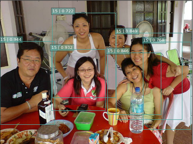
Our SSD detecotrs achieves 0.65 mAP accuracy on VOC 2007 test dataset, at the speed of 8 frames/second. Below are a few examples of detection outputs.
Here is the training/evaluation chart,
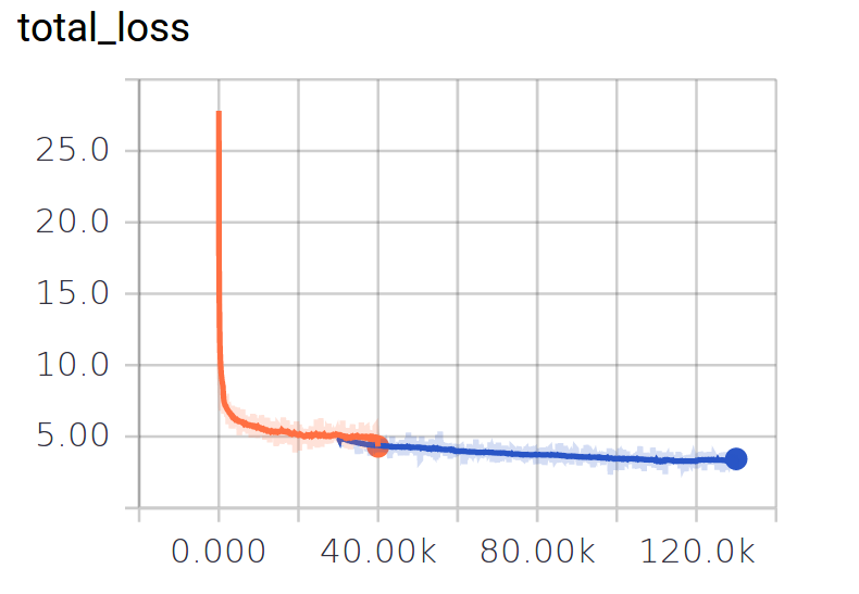
And here the loss chart.
The core of Signle Shot MultiBox Detecotr is predicting category scores and bounding boxes offsets for a fixed set of default boxes using small convolutional filters applied at features maps. For details, please refer to the original paper
Here is the model architecture for SSD. Excluding pooling, batch normalization, and dropout layers, there are 23 layers in all. Specifically, 13 VGG CNN feature layers, and 10 SSD specific detection layers.
For some of the top layers in SSD architecture, specifically, conv4,conv7,conv8,conv9,conv10,conv11, each spatial location (3x3 region) will be used to predict a fixed set of default boxes, including which classes these default boxes belong to and how much offsets these default boxes are relative to true position of the objects. There are 8732 default boxes in all.
SSD only needs an input image and ground truth boxes for each object during training. Through our matching strategy, each of the default boxes will be assigned as a class label. If they are assigned as background class, we call them negative samples. If they are assigned as non-background class, we call them positive samples. For positive samples, we will also assign bounding boxes offsets (the offsets between default box and ground truth box). Our loss function is the summary of classification loss and location loss for these samples.
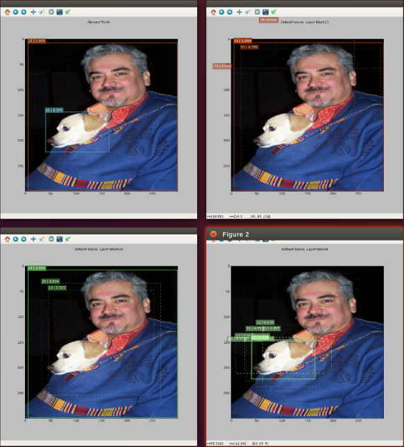
Here is an example of how some of defalut boxes are assinged as positive samples.
As mentioend earlier, VOC 2007 and VOC 2012 datasets are used in this projet, and they can be downloaded from the web.
wget http://host.robots.ox.ac.uk/pascal/VOC/voc2012/VOCtrainval_11-May-2012.tar
wget http://host.robots.ox.ac.uk/pascal/VOC/voc2007/VOCtrainval_06-Nov-2007.tar
wget http://host.robots.ox.ac.uk/pascal/VOC/voc2007/VOCtest_06-Nov-2007.tar
After downloading above datasets, we use pascalvoc_to_tfrecords.py scipt under datasets folder to convert the data into TF Records format, which will be used by our training scritp.
For example, to generate voc_train_2007 TF record files, uncomment below code lines in pascalvoc_to_tfrecords.py
#dataset_dir = "../../data/voc/2007_train/VOCdevkit/VOC2007/"
#output_dir = "../../data/voc/tfrecords/"
#name='voc_train_2007'
comment below code lines
dataset_dir = "../../data/voc/2007_test/VOCdevkit/VOC2007/"
output_dir = "../../data/voc/tfrecords/"
name='voc_test_2007'
And then execute python pascalvoc_to_tfrecords.py command in terminal. Note that you might have to modify the dataset_dir and output_dir based on where you put your dataset file, and where you want the TF records to be saved.
I conducted the training in mainly two phases:
- Overfitting the training dataset
During this phase, we mainly focus on getting high accuracy on training dataset. The purpose is to make sure that the data preparation, the model architecture, the loss function, the optimizer, the evaluation are all properly setup. The highest training mAP obtained is 0.98, This proves that, after some improvements over the baseline model implementation, our model is trainable and can converge well. - Improve result over test dataset
During this phase, we mainly focus on improving test accuracy, by means of experimentig over optimiser, batch normalization, data preparation, batch normalization, dropout and etc.
With the goal of improving testing accuracy, we conducted experimentations over various impacting aspects of the training.
A few improvements are made over baseline model so that our model implementation are consistent with the original paper.
a) strict smooth L1 loss implementation
When the regression targets are unbounded as it is the case in this project, training with L2 loss would require careful tuning of learning rates in order to prevent exploding gradients. A strict implementation of L1 loss can reduce this risk.
b) Matching strategy adjustment
As mentioned earlier, we assign each and every default box with class label and location offset based on ground truth bounding boxes. This is done by matching strategy.
In the baseline model, A default box is matched with a grounding truth bounding box if its jaccard overlap is bigger than 0.5. This has a potential problem. For some ground truth box, it might happen that its jaccard overlap with all default box are less than 0.5, as a result, these ground truth box will not be assigned to any default box, this might not be good from the perspective of training.
In our model, we correct this by strictly following the matching strategy presented in the original paper. That is, we first match each ground truth box with a default box which has biggest jaccard overlap, and then we assign default box to ground truth box which has jaccard overlap bigger than 0.5.
c) Out of bounds bounding box handling In this project, we used raddom sampling data augmentation. We randomly crop a small region of the original image to serve as our training image. As a result, ground truth box needs to be adjusted.
In the baseline, the adjustment of the ground truth bboxes is a bit inappropriate in that some of the ground truth box are out of the bounds (less than 0, or bigger than 1). Intuitively, this might make sense, but it also turns that this makes the training harder to converge. With hindsight, I think this makes training harder to converge because it’s fundamentally a harder problem in that we are required to predict the accurate position of the whole object with a partial object.
In our model, we clipped all ground truth box so that they are within [0,1] range.
Throughout the experimentations, Adam optimizer it’s used, as it implements both momentum update and per parameter adaptive learning rate.
We did experiment a lot with learning rate though. In the original paper, 0.001 learning rate is used to train SSD weights.
To my surprise, I find this does not work very well. The training took very long time to converge, and does not converge well at all. Later on I implemented batched normalization, and increased learning rate to 0.1, and this made a huge difference. With 0.1 learning rate, we are able to achieve the loss in about half an hour which would have taken 8 hours if 0.001 learning rate is used.
Three kinds of data augmentation are used, which is the same as the baseline model, except a few relevant hyperparameters.
a) flip the image horizontally
b)color distortion
Randomly change the brightness, contrast , hue and saturation of the image.
c)patch sampling
Batch normalization layers are added to the baseline model. They allowed us to use bigger learning rate and drastically reduced training time.
Drop out is also experimented in this project since we saw a large gap between training accuracy and testing accuracy. It turned out that dropout does narrow the gap between train and test accuracy, but it also dampen the training accuracy a lot. At the end, we end up with roughly the same test accuracy with or without dropout.
Training experimentation and progress are logged in history/notes.txt file. Below are a quick summary:
- Fix bugs in baseline made the model converge
- Batch normalization and bigge learning rate made a huge difference. traning accuray from 0.8 to 0.98
- Data augmenation is very effective in improving testing accuray, from 0.5 to 0.65
Current implementation can do a decent detection job. but its performance can be further improved on some images, like below,
In the original paper, the test accuracy is 0.69. If we could push our current test accurcy from 0.65 to 0.69 or higher, we should be able to have better detection result. I think the key should lie in how we perform data augmentation,
- Replicate the reference data augmentation implementation as much as possible
Our current implementation already try to closely follow the instruction of the original paper regarding data augmenation. But we implemented with python and tensorflow, while the original paper implemented with c++, caffe and opencv. There should be some difference between the two implementations that is causeing the test accuracy gap. - Add zoom out operation
SSD is known to have relatively poor performance on detecitng small objects (like bottle,pottedplant), as also confirmed by our SSD implementation. So one idea to improve is to add more small objects to training data by performing zoom out operation during data augmentation.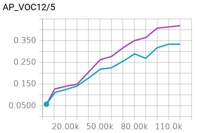
- Python 3.5
- Tensorflow 1.0.0
The training took about 58 hours on a Nvidia GTX 1080 GPU.
run python ./train_model.py with below setting
self.max_number_of_steps = 30000
self.learning_rate = 0.1
self.fine_tune_vgg16 = False
1). Run python ./train_model.py with below setting
Before you run the ./train_model.py script, you will have to download the vgg16 pretrained weigths from here to a local folder, change the setting of self.checkpoint_path if necessary.
self.checkpoint_path = '../data/trained_models/vgg16/vgg_16.ckpt'
self.fine_tune_vgg16 = True
self.max_number_of_steps = 900000
self.learning_rate=0.01
2). Run python ./train_model.py with below setting
self.fine_tune_vgg16 = True
self.max_number_of_steps = 1100000
self.learning_rate=0.001
3). Run python ./train_model.py with below setting
self.fine_tune_vgg16 = True
self.max_number_of_steps = 1200000
self.learning_rate=0.0005
1). Run python ./run_all_checkpoints.py with below settings
min_step = 100
step = 10000
2). Run python ./run_all_checkpoints.py -f with below settings
min_step = 30000
step = 10000
