- About this project
- Controls
- How to run the project
- Program arguments
- Available versions
- Available initializations
- Program structure
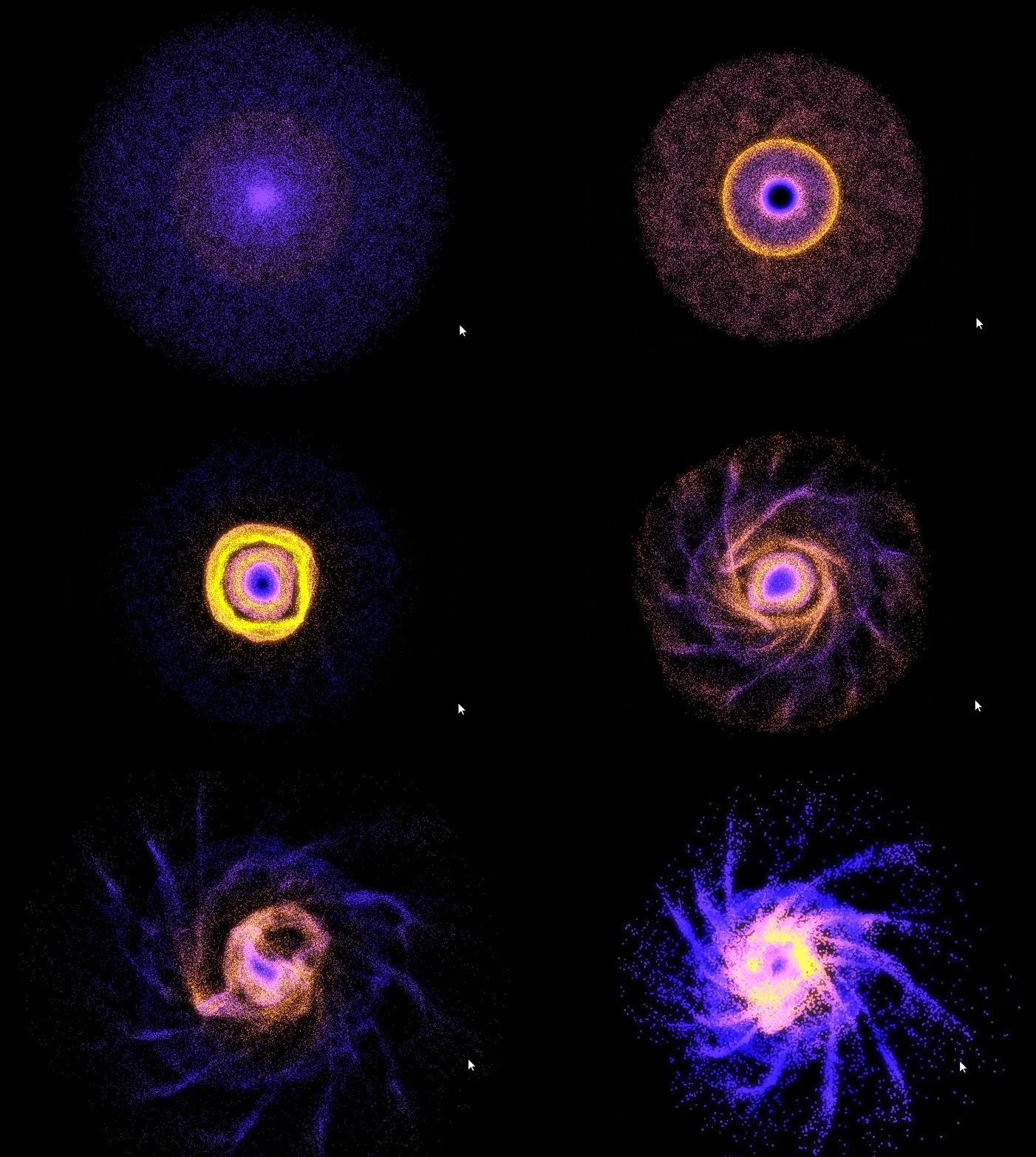
This project was made to learn C++, OpenGL and GPU programming.
- Different versions/algorithms can be tried.
- Different initializations can be tried.
- The number of bodies to simulate can be customized.
- The simulation is in a 3D world.
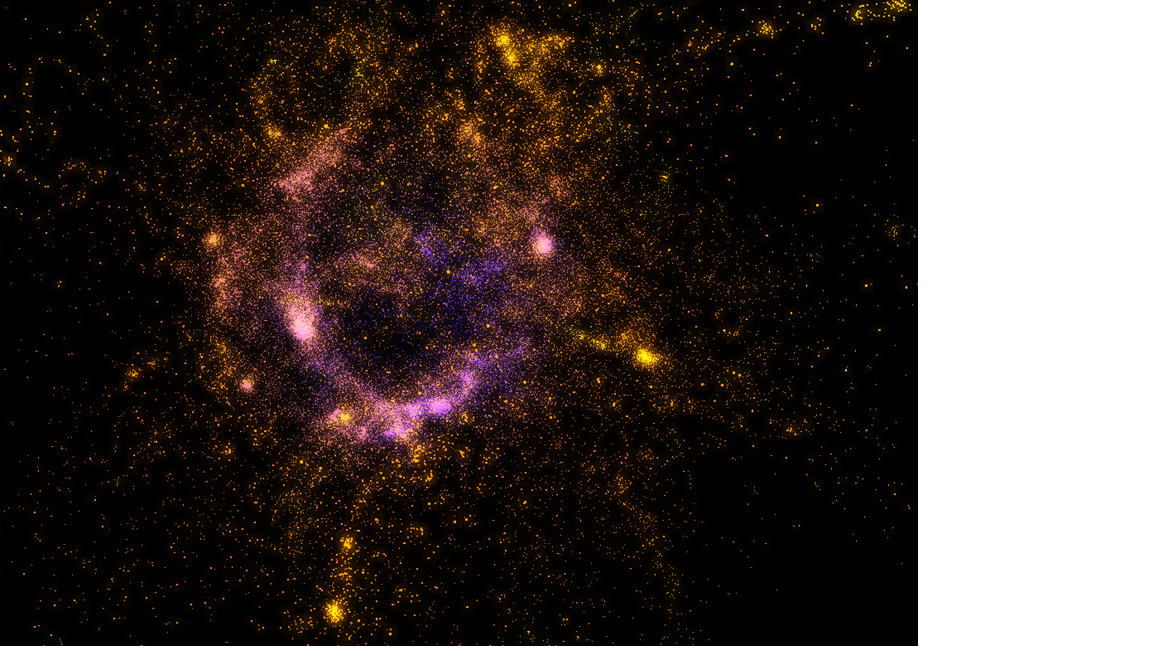
- Particles have bloom.
- Leapfrog integrator.
- Plummer softening.
- Customizable step size and squared softening.
| Key/Input | Action |
|---|---|
| Esc | Close the program |
| Space | Pause/start the simulation |
| Mouse scroll | Zoom in/out |
| Click and drag | Move the camera |
| B | Activate/Deactivate bloom |
| I | Increase bloom intensity |
| D | Decrease bloom intensity |
| Q | Enable/disable point size |
| S | Save the current state of the simulation |
You need to have installed:
gitxorg-devcmakemake
This command will create a new directory titled build and change the location to it.
mkdir build && cd buildBuild a Makefile using cmake.
cmake ..Compile the program using the Makefile.
makeRun the compiled program.
./N-bodygitcmakemingw
Since the program uses OpenMP, you also need to install this:
mingw-get install mingw32-pthreads-w32
These commands will create a new directory titled build and change the location to it.
mkdir build
cd build
Build a Makefile using cmake.
cmake -G "MinGW Makefiles" ..Compile the program using the Makefile.
mingw32-makeRun the compiled program.
.\N-body.exe -v (number)Configure which version you want to use.-i (number)Configure which initialization you want (How the bodies are initialized).-n (number)Configure how many bodies you want to simulate.-t (decimalNumber)Configure the step size. (Smaller the more precise)-s (decimalNumber)Configure the squared softening.-f (path/to/file)Provide a particle system file.-o (customFileName)Save the simulation.
The default arguments are:
./N-body -v 1 -i 2 -n 100 -t 0.0035 -s 40.0Alternative usage:
./N-body -version 1 -init 2 -n 100 -time-step 0.0035 -softening 40.0These are the available versions you can try:
-v 1Particle-particle sequential algorithm (n^2 complexity) using the CPU.-v 2Particle-particle parallel algorithm (n^2 complexity) using the CPU (OpenMP).-v 3Particle-particle parallel algorithm (n^2 complexity) using the GPU (Compute shaders).-v 4Optimized version 3. Implementation of Nvidia - Fast N-body simulation. (Compute shaders)-v 5Fixed grid algorithm CPU parallel.
You can try the next initializations:
-i 1Particles form a cube.-i 2Particles form a disk.-i 3Particles form an equilateral triangle. (Only 3 particles)-i 4Particles form a sphere. (Only the surface)-i 5Particles form a ball.-i 6Particles form a cube. (Only the surface)
The files you give to the program must follow this format:
Particle System with 3 particles:
Particle ID: 0
Position: (5.8337, 4.6008, 3.35599)
Velocity: (-1.15428, 1.8317, 0)
Acceleration: (0, 0, 0)
Mass: 0.625
Particle ID: 1
Position: (2.13544, 2.37607, 3.12727)
Velocity: (1.01254, -1.94254, 0)
Acceleration: (0.4, 3.0, 0)
Mass: 0.875
Particle ID: 2
Position: (2.74389, 2.46503, 3.42229)
Velocity: (0.0960527, 2.17343, 0)
Acceleration: (0, 0, -8.0)
Mass: 0.875
Particle ID: 3
Position: (3.38766, 0.977181, 2.78489)
Velocity: (1.10174, 2.40912, 0)
Acceleration: (-8.0, 0, 0)
Mass: 0.625
Note: The world dimensions are (5, 5, 5)
This is how you can use the -f argument:
./N-body -f path/to/fileThe program offers the ability to save various states of the simulation. It includes the following features:
- Saving the initial state: The program automatically saves the initial state at the start of the simulation.
- Saving the current state: By pressing the "S" key during the simulation, you can save the current state for later analysis.
- Saving the final state: At the end of the simulation, the program saves the final state.
The saved states are stored in files located in the compiled directory of the program. To save the states, you need to provide a filename using the -output or -o argument when running the program.
These saving functionalities allow capturing different moments of the simulation for further analysis and study.
There's a benchmark (written in Python) available for measuring the performance of each version, which generates different plots for comparison. If you're interested, please read the readme file inside the benchmark directory.
Here you can see the class diagram. It should be relativley easy to add new initializations and versions.
An example of how a new simulation version can be added is by creating a new class that implements the ParticleSolver interface and then including the new version in the list of available version options in the ArgumentsParser class. This way, the user can select the new version through the input arguments.
Similarly, to add a new initialization, a new class that implements the ParticleSystemInitializer interface can be created and the new option can be added to the list of initialization options in the ArgumentsParser class.
Finally, you would have to use the new initalization or version you created in main.cpp.


