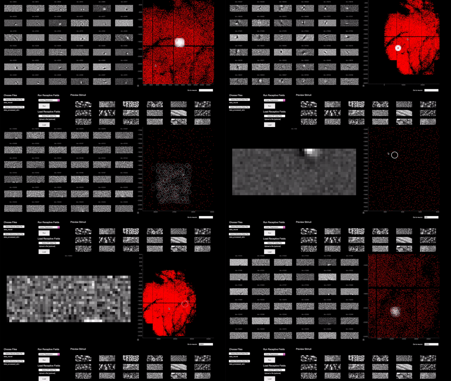
GUI to compute and explore receptive fields, primarily from calcium imaging recordings.
You can run the GUI, or alternatively, you can investigate the Jupyter notebooks that use its functionality.
The GUI is based in PyQt and runs on Python 3.
This repository was made by Sonia Joseph (GitHub, Twitter) at the Stringer Lab at Janelia Research Campus in Spring 2021.
Pull requests are welcome for bug fixes and additional features!
This repository runs on Python 3, so make sure that is installed first. Clone repository from GitHub install requirements, and run.
# Clone git repo
git clone https://github.com/MouseLand/receptivefield-explorer

# Enter directory
cd receptivefield-explorer

# Create a virtual environment to contain the requirements
python3 -m venv env

# Install requirements
pip3 install -r requirements.txt

# From outside the directory, run the RF-explorer
cd ..
python3 -m receptivefield-explorer
The neural data file should be an .npz file in dictionary format with the following keys, containing array data with these shapes:
dat['istim']: <class 'numpy.ndarray'> (13860,)
dat['frame_start'] <class 'numpy.ndarray'> (13860,)
dat['ypos'] <class 'numpy.ndarray'> (100,)
dat['xpos'] <class 'numpy.ndarray'> (100,)
dat['spks'] <class 'numpy.ndarray'> (100, 29800) # neural data in neurons x timepoints
The spk data will be processed according to 'istim' and 'frame_start' and then Z-scored. The retinotopy will automatically be graphed using the 'xpos' and 'ypos' information.
The stimulus data should be in a .mat file in dictionary format with 'img' as a key. dat['img'] contains stimuli data in shape height x width x number of stimuli.
dat['img']: <class 'numpy.ndarray'> (150, 400, 16000)
Downsampling the data will make the stimuli smaller, which speeds up the receptive field calculation. The data is by default downsized to (18, 48), but change the specifications to your preferences using the downsample height and width boxes.
You have the option to use a linear regression or reduced rank regression. Press Run. Note that this computation involves large matrix multiplications and may be slow without GPU.
Alternatively, you can load precomputed RFs. Receptive fields will be in a dictionary containing keys 'B0' and 'Spred,' where B0 is a matrix of receptive fields for all neurons, and Spred are predicted spikes.
Click on a neuron or multiple neurons in the retinotopy to bring up the corresponding receptive fields.
If you hold down Command on Mac or Control on Windows while clicking neurons on the retinotopy, you can view multiple receptive fields at a time.
You can zoom in and out of the retinotopy to achieve more or less precision for the number of neurons that you select.
The /notebooks folder contains sample notebooks demo-ing transformations on neural data.
- neural encoding model training - trains a simple CNN and a multi-layer CNN to predict neural response based on sample data. The trained models can then be used in the maximally activating stimulus notebook.
- maximally activating stimuli - uses gradient ascent on a pre-trained deep neural encoding model to generate "maximally activating stimuli" for a particular neuron.
- receptive fields - calculates receptive fields based off linear methods like linear regression and reduced rank regression.
