Thompson et. al. 2020, Data and Code Repository

Neil F. Thompson, Eric C. Anderson, Anthony Clemento, Matthew Campbell, Devon E. Pearse, James Hearsey, Andrew P. Kinziger, John Carlos Garza

Last Updated: 2020-05-15

This repository includes code, data, and some intermediate results to reproduce the results in Thompson et al. (“A complex phenotype in salmon controlled by a simple change in migratory timing”). You can get the whole thing by cloning or downloading the repo from https://github.com/eriqande/thompson-et-al-2020-chinook-salmon-migration-timing.

If you are viewing this as the README of a GitHub repository, note that you can read it in a somewhat friendlier format (i.e., with a table of contents, etc.) on GitHub pages at: https://eriqande.github.io/thompson-et-al-2020-chinook-salmon-migration-timing/

For the whole-genome resequencing data, the production of BAMs and VCFs from the original FASTQ files follows a standard bwa/GATK pipeline as described in the supplemental methods. Here we focus on analyses of the products of that work. The various steps are described in a series of RMarkdown documents with a fair bit of explanation/description of the procedures. Analyses requiring the use of cluster computing resources are described and documented, but will not be run automatically by evaluating the RMarkdown document. Implementing them yourself will require modification for the vagaries of your own high performance computing system and preferred mode of parallelization, etc. Running some of the RMarkdown documents requires a proper shell. These were initially developed and run on a Mac. They have also been tested and confirmed to run on a server running CentOs 7.

Rmarkdown documents in the 000 series were developed primarily by Eric C. Anderson. Rmarkdown documents in the 100 series were developed primarily by Neil F. Thompson. Rmarkdown documents in the 200 series were developed primarily by Eric C. Anderson and deal with further analyses done to respond to several reviewer queries.

In most cases, products from cluster computing are placed in this repository within the stored_results directory. This means that all the RMarkdown documents can be evaluated successfully without first running the cluster-based analyses, except for 002-allele-frequencies.Rmd, for which the products from the cluster-based analyses require too much space to store in this repository. Fortunately, none of the downstream analyses depend upon the outputs from 002-allele-frequencies.Rmd.

All the RMarkdown documents can be evaluated en masse (except for 002-allele-frequencies.Rmd) by sourcing the R script render-numbered-Rmds.R. On a fairly old mac laptop the run times for each are as follows. Note that this does not include the time required to create the stored results on the cluster, etc.

Rmarkdown document	Run time
001-align-coho-genome.Rmd	1.7 secs
002-allele-frequencies.Rmd (after running initial results on cluster)	3.3 mins
003-extract-johnson-creek-variants.Rmd	8.7 mins
004-prepare-haplotypes.Rmd	11.2 mins
005-annotating-variants-near-greb1l.Rmd	5.9 mins
006-haplo-raster-plots.Rmd	1.2 mins
007-arg-inference-and-plotting.Rmd	4.9 mins
008-read-depths-and-duplications.Rmd	41.2 secs
009-rosa-dna-distance-trees.Rmd	2.3 mins
010-salmon-river-carcasses.Rmd	48.2 secs
011-recombinant-frequencies.Rmd	1.5 mins
012-coalescent-modeling-of-recombinants.Rmd	3.5 mins
100-RoSA-figure1-map.Rmd	16.4 secs
101-Klamath-estuary-GSI-rubias.Rmd	18.0 secs
102-Klamath-estuary-ANOVA-sampling-date-RoSA.Rmd	11.0 secs
102.1-Klamath-estuary-partial-correlation.Rmd	1.6 secs
103-Klamath-estuary-GonadSI-mixed-model-analysis.Rmd	3.3 secs
103.1-Klamath-estuary-GonadSI-power-analysis.Rmd	1.4 mins
104-Klamath-estuary-nonwaterfraction-adiposity-mixed-model-analysis.Rmd	2.1 secs
104.1-Klamath-estuary-nonwaterfraction-power-analysis.Rmd	1.7 mins
105-Klamath-estuary-figure4.Rmd	7.7 secs
106-TrinityRiver-ANOVA-etc.Rmd	9.5 secs
107-RoSA-population-genetics-survey.Rmd	1.6 secs
108-Klamath-basin-early-RoSA-haplotype-abundance-commercial-fishery-model-tableS10.Rmd	1.2 secs
201-01-prep-bams-to-seek-inversions.Rmd	0.16 secs
201-02-seek-inversions.Rmd	3.7 mins
201-03-seek-inversions-with-gridss.Rmd	4.0 secs
202-01-genomewide-allele-freqs-from-the-bams.Rmd	4.7 secs
203-01-pca-for-gwas-covariate.Rmd	4.7 secs
203-02-gwas-with-angsd.Rmd	4.4 mins
204-01-assess-genotyping-error-rate-with-whoa.Rmd	1.2 mins
204-02-assess-genotype-error-from-subsampled-hi-read-depth-samples.Rmd	2.0 mins
204-03-simulate-imputation-and-phasing-error-for-trees.Rmd	6.7 mins

Preliminaries and Dependencies

Below is a description of the needed dependencies. A script to install all of them on one of our test clusters is at 000-00-prepare-dependencies.sh, but it will likely need some tweaking on your system.

Genomes, etc.

Download the necessary Chinook and coho genomes and put them in a new directory called genome in this repository. Index them with samtools faidx.

mkdir genome
cd genome

# coho genome
wget ftp://ftp.ncbi.nlm.nih.gov/genomes/all/GCF/002/021/735/GCF_002021735.1_Okis_V1/GCF_002021735.1_Okis_V1_genomic.fna.gz
mv GCF_002021735.1_Okis_V1_genomic.fna.gz Okis_V1_genomic.fna.gz
gunzip Okis_V1_genomic.fna.gz 
samtools faidx Okis_V1_genomic.fna


# chinook genome
wget ftp://ftp.ncbi.nlm.nih.gov/genomes/all/GCF/002/872/995/GCF_002872995.1_Otsh_v1.0/GCF_002872995.1_Otsh_v1.0_genomic.fna.gz
mv GCF_002872995.1_Otsh_v1.0_genomic.fna.gz Otsh_V1_genomic.fna.gz
gunzip Otsh_V1_genomic.fna.gz 
samtools faidx Otsh_V1_genomic.fna

# chinook genome GFF
wget ftp://ftp.ncbi.nlm.nih.gov/genomes/all/GCF/002/872/995/GCF_002872995.1_Otsh_v1.0/GCF_002872995.1_Otsh_v1.0_genomic.gff.gz

# Narum et al. version of Chinook genome from the Johnson Creek fish
wget ftp://ftp.ncbi.nlm.nih.gov/genomes/genbank/vertebrate_other/Oncorhynchus_tshawytscha/all_assembly_versions/GCA_002831465.1_CHI06/GCA_002831465.1_CHI06_genomic.fna.gz
gunzip GCA_002831465.1_CHI06_genomic.fna.gz
samtools faidx GCA_002831465.1_CHI06_genomic.fna

cd ../

Geospatial data

Make a directory in the top level of the repository called geo-spatial and then put some things in there:

Get CalWater2.2.1 by going to https://drive.google.com/file/d/13WqsA3jK1C0kW5zaznEwDkg3wBc-cBco/view and then choosing the Google Drive download button to download a whole zip file that expands into a directory named GISlayers_calw221_shp. Move or symlink that whole directory inside geo-spatial. These are watershed boundaries.
Get California stream line data from http://data-cdfw.opendata.arcgis.com/datasets/29c40f65341749b3aa26d3f0e09502b9_4.zip. Unzip that directory into one called California_Streams and move or symlink that directory into geo-spatial.
Download some things from Natural Earth Data:
- Natural Earth II with Shaded Relief, Water, and Drainages raster https://www.naturalearthdata.com/http//www.naturalearthdata.com/download/10m/raster/NE2_HR_LC_SR_W_DR.zip. Put or symlink the resulting directory, NE2_HR_LC_SR_W_DR into geo-spatial.
- 10m-cultural-vectors, Admin 1 – States, Provinces, Download boundary lines: https://www.naturalearthdata.com/http//www.naturalearthdata.com/download/10m/cultural/ne_10m_admin_1_states_provinces_lines.zip. Put or symlink the resulting directory, ne_10m_admin_1_states_provinces_lines into geo-spatial.
- Finally, get the coastlines: https://www.naturalearthdata.com/http//www.naturalearthdata.com/download/10m/physical/ne_10m_coastline.zip, and put the resulting folder, ne_10m_coastline into geo-spatial.

Unix Programs

The following programs must be installed and available in the PATH. Versions used on Eric’s laptop appear in parentheses.

angsd (Version: 0.920, using htslib: 1.6)
bwa (Version: 0.7.16a-r1181)
samtools (Version: 1.3, using htslib 1.3)
bcftools (Version: 1.9, using htslib 1.9)
bgzip, tabix (Version 1.6) These are found within the htslib library.
vcftools (Version v0.1.12b)
bedtools (Version v2.27.1)
PHASE (Version 2.1.1)

lastz (Version 1.04) This was obtained and compiled thus:

wget http://www.bx.psu.edu/~rsharris/lastz/lastz-1.04.03.tar.gz
gunzip lastz-1.04.03.tar.gz
tar -xvf lastz-1.04.03.tar
cd lastz-distrib-1.04.03/
make
make install

maf2fasta, single_cov2 (From multiz Version 012109) Obtain and compile like this:

wget http://www.bx.psu.edu/miller_lab/dist/multiz-tba.012109.tar.gz
gunzip multiz-tba.012109.tar.gz
tar -xvf multiz-tba.012109.tar
cd multiz-tba.012109/
make

Java jars

The following Java-based programs must be downloaded, and the paths to their associated Jar files must be listed appropriately in the file script/java-jar-paths.R:

BEAGLE. (Version 4.1) The version here is important. Don’t use version 5.
RentPlus (Version v0.5)

The distributed version of script/java-jar-paths.R reflects the placement of Jar files on Eric’s system:

# central place in repository to store paths for Java Jar files we use

BEAGLE=/Users/eriq/Documents/others_code/BEAGLE_4.1/beagle.27Jan18.7e1.jar
RentPlus=/Users/eriq/Documents/others_code/RentPlus/RentPlus.jar

This should be updated to reflect where you have stored the jar files on your system.

One more Java program—snpEff—is required. The installation procedure for this is slightly different, owing to it needing to store data bases in the directory where the Jar file resides (apparently).

So,

Download snpEff The link provided is for Version 4.3 with a release date of 24 November 2017. THis is the version we used.
Expand that zip archive and move the resulting directory into
the top level of this repository. When you are done, you should be able to ls the Jar file like this:

ls snpEff_v4_3t_core/snpEff/snpEff.jar

R Packages

Packages must be downloaded from CRAN, BioConductor, and GitHub. The following code, which is in R/install_packages_etc.R, will download and install the necessary packages:

# just R code to install the packages needed for running the notebooks

# get the packages needed from CRAN
install.packages(
  c(
    "ape",
    "broom",
    "callr",
    "car",
    "cowplot",
    "ggsn",
    "ggspatial",
    "kableExtra",
    "knitr",
    "lubridate",
    "maps",
    "mapproj",
    "nlme",
    "pander",
    "parallel",
    "phangorn",
    "plotly",
    "ppcor",
    "raster",
    "remotes",
    "rmarkdown",
    "rubias",
    "sessioninfo",
    "sf",
    "sjPlot",
    "tidyverse",
    "vcfR",
    "viridis",
    "whoa",
    "zoo"
  ),
  repos = "http://cran.rstudio.com"
)

# Note that, on the cluster, since I don't have admin access,
# I needed to get the sysadmin to get rgdal installed and to
# install libudunits2.so in order to complete the install of:
# units, rgdal, sf, rosm, lwgeom, ggsn, ggspatial



# get the packages needed from BioConductor
if (!requireNamespace("BiocManager", quietly = TRUE)) {
  install.packages("BiocManager", repos = "http://cran.rstudio.com")
}

BiocManager::install("ggtree")
BiocManager::install("treeio")


# Get package ecaRbioinf at https://github.com/eriqande/ecaRbioinf
# This is a package of useful functions by Eric C. Anderson. We
# used commit `6972defd`.  Get it like this:
remotes::install_github("eriqande/ecaRbioinf", ref = "6972defd")

RMarkdown Documents

The following RMarkdown documents should be evaluated in order. The script render-numbered-Rmds.R will do that (except for 002-allele-frequencies.Rmd) when run in the top level of this repository. Some RMarkdown documents rely on outputs from previous ones. Some of these RMarkdown documents include calls to Unix utilities, so might not run on non-Unix or non-Linux architectures.

Outputs (figures, tables, R data objects, etc) from each RMarkdown document are written to the outputs/XXX directories. Intermediate files written during evaluation of each RMarkdown document are written to the intermediates/XXX directories. To facilitate working between the cluster and a desktop/laptop, some outputs are written to the stored_results/XXX directories which are version controlled and included in this repo.

Thumbnails of the figures and tables generated by each RMarkdown document appear below. Additionally, at the top of each section is a link to the compiled (HTML-version) of the RMarkdown document on GitHub Pages.

001-align-coho-genome.Rmd

(Compiled RMarkdown HTML document on GitHub Pages: 001-align-coho-genome.html)

The products of this analysis go into creation of some of the trees (009) and also in the designation of the alleles as ancestral or not in some of the haplotype rasters (006).

002-allele-frequencies.Rmd

(Compiled RMarkdown HTML document on GitHub Pages: 002-allele-frequencies.html)

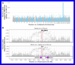
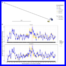
Calculation of allele frequency differences between early- and late-running forms across the genome, and around GREB1L, and the generation of plots.

003-extract-johnson-creek-variants.Rmd

(Compiled RMarkdown HTML document on GitHub Pages: 003-extract-johnson-creek-variants.html)

Using the previously assembled Chinook salmon genome from Narum et al. (2018) to ascertain variation from that Upper Columbia River summer/spring-run fish around the GREB1L region. The products of this analysis go into some later trees and haplotype rasters.

004-prepare-haplotypes.Rmd

(Compiled RMarkdown HTML document on GitHub Pages: 004-prepare-haplotypes.html)

Using BEAGLE to impute genotypes and infer haplotypes in 5 Mb around GREB1L. The outputs of this analysis are used for a number of downstream analyses.

005-annotating-variants-near-greb1l.Rmd

(Compiled RMarkdown HTML document on GitHub Pages: 005-annotating-variants-near-greb1l.html)

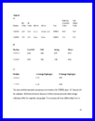
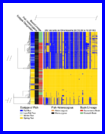
Using snpEff to annotate variants and then analyzing a few of them. This provides data that goes into Table S1 (“Two near-perfectly associated, non-synonymous variants in the GREB1L gene”), and is also used later for the haplotype raster plots.

006-haplo-raster-plots.Rmd

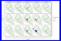
(Compiled RMarkdown HTML document on GitHub Pages: 006-haplo-raster-plots.html)

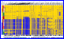
Compiling some auxiliary information (gene/exon inclusion, etc.) and then making haplotype raster plots using functions from the ‘ecaRbioinf’ package.

007-arg-inference-and-plotting.Rmd

(Compiled RMarkdown HTML document on GitHub Pages: 007-arg-inference-and-plotting.html)

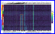
Using RENT+ (Mirzaei and Wu 2016) to infer the ancestral recombination graph in the RoSA and plot it with a tree/heatmap, using ggtree (Yu et al. 2017).

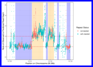
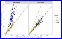
008-read-depths-and-duplications.Rmd

(Compiled RMarkdown HTML document on GitHub Pages: 008-read-depths-and-duplications.html)

Using bedtools to compute read depths from the BAMs and then demonstrate that the apparent duplications are highly associated with run type.

009-rosa-dna-distance-trees.Rmd

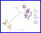
(Compiled RMarkdown HTML document on GitHub Pages: 009-rosa-dna-distance-trees.html)

Making distance trees between haplotypes in the RoSA region, and including coho salmon.

010-salmon-river-carcasses.Rmd

(Compiled RMarkdown HTML document on GitHub Pages: 010-salmon-river-carcasses.html)

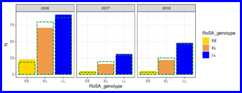
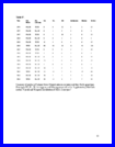
Genotype frequency, spatial and temporal analyses of RoSA genotypes of post-spawn Salmon River carcasses. Data from here also go into Table S7 (“Summary of number of Salmon River Chinook salmon carcasses and their RoSA genotypes”).

011-recombinant-frequencies.Rmd

(Compiled RMarkdown HTML document on GitHub Pages: 011-recombinant-frequencies.html)

Determining frequencies of recombinant haplotypes between the RoSA region and the imperfectly associated SNPs reported in Prince et al. (2017). Data from this RMarkdown document go into Table S9 (“Frequencies of haplotypes recombinant/non-recombinant between the distal and RoSA region in collections from California and Oregon”).

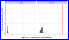
012-coalescent-modeling-of-recombinants.Rmd

(Compiled RMarkdown HTML document on GitHub Pages: 012-coalescent-modeling-of-recombinants.html)

Performing discrete-time, coalescent-with-recombination simulations to determine whether we expect to see such a high recombinant frequency in the Klamath River — Iron Gate Hatchery collection if spring-fall introgression only occurred after human modifications to the watershed.

100-RoSA-figure1-map-using-sf.Rmd

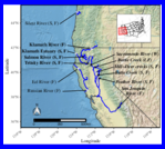
(Compiled RMarkdown HTML document on GitHub Pages: 100-RoSA-figure1-map-using-sf.html)

Making the map for Figure 1.

101-Klamath-estuary-GSI-rubias.Rmd

(Compiled RMarkdown HTML document on GitHub Pages: 101-Klamath-estuary-GSI-rubias.html)

Genetic stock identification of Chinook salmon caught in the Klamath River estuary.

102-Klamath-estuary-ANOVA-sampling-date-RoSA.Rmd

(Compiled RMarkdown HTML document on GitHub Pages: 102-Klamath-estuary-ANOVA-sampling-date-RoSA.html)

103-Klamath-estuary-GonadSI-mixed-model-analysis.Rmd

(Compiled RMarkdown HTML document on GitHub Pages: 103-Klamath-estuary-GonadSI-mixed-model-analysis.html)

103.1-Klamath-estuary-GonadSI-power-analysis.Rmd

(Compiled RMarkdown HTML document on GitHub Pages: 103.1-Klamath-estuary-GonadSI-power-analysis.html)

104-Klamath-estuary-nonwaterfraction-adiposity-mixed-model-analysis.Rmd

(Compiled RMarkdown HTML document on GitHub Pages: 104-Klamath-estuary-nonwaterfraction-adiposity-mixed-model-analysis.html)

104.1-Klamath-estuary-nonwaterfraction-power-analysis.Rmd

(Compiled RMarkdown HTML document on GitHub Pages: 104.1-Klamath-estuary-nonwaterfraction-power-analysis.html)

105-Klamath-estuary-figure4.Rmd

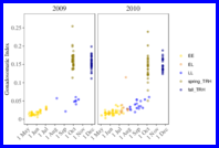
(Compiled RMarkdown HTML document on GitHub Pages: 105-Klamath-estuary-figure4.html)

106-TrinityRiver-ANOVA-etc.Rmd

(Compiled RMarkdown HTML document on GitHub Pages: 106-TrinityRiver-ANOVA-etc.html)

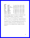
107-RoSA-population-genetics-survey.Rmd

(Compiled RMarkdown HTML document on GitHub Pages: 107-RoSA-population-genetics-survey.html)

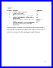
108-Klamath-basin-early-RoSA-haplotype-abundance-commercial-fishery-model-tableS10.Rmd

(Compiled RMarkdown HTML document on GitHub Pages: 108-Klamath-basin-early-RoSA-haplotype-abundance-commercial-fishery-model-tableS10.html)

201-01-prep-bams-to-seek-inversions.Rmd

(Compiled RMarkdown HTML document on GitHub Pages: 201-01-prep-bams-to-seek-inversions.html)

201-02-seek-inversions.Rmd

(Compiled RMarkdown HTML document on GitHub Pages: 201-02-seek-inversions.html)

201-03-seek-inversions-with-gridss.Rmd

(Compiled RMarkdown HTML document on GitHub Pages: 201-03-seek-inversions-with-gridss.html)

202-01-genomewide-allele-freqs-from-the-bams.Rmd

(Compiled RMarkdown HTML document on GitHub Pages: 202-01-genomewide-allele-freqs-from-the-bams.html)

203-01-pca-for-gwas-covariate.Rmd

(Compiled RMarkdown HTML document on GitHub Pages: 203-01-pca-for-gwas-covariate.html)

203-02-gwas-with-angsd.Rmd

(Compiled RMarkdown HTML document on GitHub Pages: 203-02-gwas-with-angsd.html)

204-01-assess-genotyping-error-rate-with-whoa.Rmd

(Compiled RMarkdown HTML document on GitHub Pages: 204-01-assess-genotyping-error-rate-with-whoa.html)

204-02-assess-genotype-error-from-subsampled-hi-read-depth-samples.Rmd

(Compiled RMarkdown HTML document on GitHub Pages: 204-02-assess-genotype-error-from-subsampled-hi-read-depth-samples.html)

204-03-simulate-imputation-and-phasing-error-for-trees.Rmd

(Compiled RMarkdown HTML document on GitHub Pages: 204-03-simulate-imputation-and-phasing-error-for-trees.html)

References

Mirzaei, Sajad, and Yufeng Wu. 2016. “RENT+: An Improved Method for Inferring Local Genealogical Trees from Haplotypes with Recombination.” Bioinformatics 33 (7). Oxford University Press: 1021–30.

Narum, Shawn R., Alex Di Genova, Steven J. Micheletti, and Alejandro Maass. 2018. “Genomic Variation Underlying Complex Life-History Traits Revealed by Genome Sequencing in Chinook Salmon.” Proceedings of the Royal Society B: Biological Sciences 285 (1883): 20180935. https://doi.org/10.1098/rspb.2018.0935.

Prince, Daniel J., Sean M. O’Rourke, Tasha Q. Thompson, Omar A. Ali, Hannah S. Lyman, Ismail K. Saglam, Thomas J. Hotaling, Adrian P. Spidle, and Michael R. Miller. 2017. “The Evolutionary Basis of Premature Migration in Pacific Salmon Highlights the Utility of Genomics for Informing Conservation.” Science Advances 3 (8): e1603198. https://doi.org/10.1126/sciadv.1603198.

Yu, Guangchuang, David K. Smith, Huachen Zhu, Yi Guan, and Tommy Tsan-Yuk Lam. 2017. “Ggtree: An R Package for Visualization and Annotation of Phylogenetic Trees with Their Covariates and Other Associated Data.” Methods in Ecology and Evolution 8 (1): 28–36. https://doi.org/10.1111/2041-210X.12628.

NotebookOFXiaoMing/thompson-et-al-2020-chinook-salmon-migration-timing