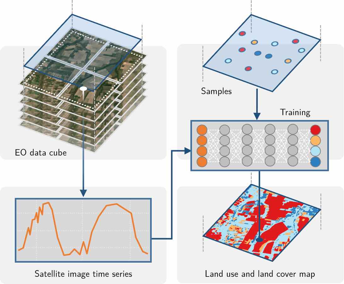
sits is an open source R package for satellite image time series
analysis. It enables users to apply machine learning techniques for
classifying image time series obtained from earth observation data
cubes. The basic workflow in sits is:
- Select an image collection available on cloud providers AWS, Microsoft Planetary Computer, Digital Earth Africa, Swiss Data Cube, NASA Harmonized Landsat/Sentinel and Brazil Data Cube.
- Build a regular data cube from analysis-ready image collections.
- Extract labelled time series from data cubes to be used as training samples.
- Perform samples quality control using self-organised maps.
- Train machine learning and deep learning models.
- Tune deep learning models for improved accuracy.
- Classify data cubes using machine learning and deep learning models.
- Run spatial-temporal segmentation methods for object-based time series classification.
- Post-process classified images with Bayesian smoothing to remove outliers.
- Estimate uncertainty values of classified images.
- Evaluate classification accuracy using best practices.
- Improve results with active learning and self-supervised learning methods.
Detailed documentation on how to use sits is available in the e-book
“Satellite Image Time Series Analysis on Earth Observation Data
Cubes”.
Those that want to evaluate the sits package before installing are
invited to run the examples available on
Kaggle. If you are new on
kaggle, please follow the
instructions
to set up your account. These examples provide a fast-track introduction
to the package. We recommend running them in the following order:
- Introduction to SITS
- Working with time series in SITS
- Creating data cubes in SITS
- Improving the quality of training samples
- Machine learning for data cubes
- Classification of raster data cubes
- Bayesian smoothing for post-processing
- Uncertainty and active learning
- Object-based time series classification
The sits package relies on the geospatial packages sf, stars,
gdalcubes and terra, which depend on the external libraries GDAL and
PROJ. Please follow the instructions for installing sits from the
Setup chapter of the on-line sits
book.
sits can be installed from CRAN:
install.packages("sits")The latest supported version is available on github. It may have additional fixes from the version available from CRAN.
devtools::install_github("e-sensing/sits", dependencies = TRUE)# load the sits library
library(sits)
#> SITS - satellite image time series analysis.
#> Loaded sits v1.4.2-1.
#> See ?sits for help, citation("sits") for use in publication.
#> Documentation avaliable in https://e-sensing.github.io/sitsbook/.Classification using torch-based deep learning models in sits uses
CUDA compatible NVIDIA GPUs if available, which provides up 10-fold
speed-up compared to using CPUs only. Please see the installation
instructions for
more information on how to install the required drivers.
Users create data cubes from analysis-ready data (ARD) image collections
available in cloud services. The collections accessible in sits
1.4.2.1 are:
- Brazil Data Cube (BDC): Open data collections of Sentinel-2, Landsat-8 and CBERS-4 images.
- Microsoft Planetary Computer (MPC): Open data collection of Sentinel-2/2A and Landsat-8
- Earth on AWS (AWS): Sentinel-2/2A level 2A collections.
- Digital Earth Africa (DEAFRICA): Open data collection of Sentinel-2/2A and Landsat-8 for Africa.
- USGS: Landsat-4/5/7/8 collections, which are not open data.
- Swiss Data Cube (SDC): Open data collection of Sentinel-2/2A and Landsat-8.
- NASA Harmonized Landsat/Sentinel Collection HLS.
Open data collections do not require payment of access fees. Except for those in the Brazil Data Cube, these collections are not regular. Irregular collections require further processing before they can be used for classification using machine learning models.
The following code defines an irregular data cube of Sentinel-2/2A
images available in the Microsoft Planetary Computer, using the open
data collection "SENTINEL-2-L2A". The geographical area of the data
cube is defined by the tiles "20LKP" and "20LLKP", and the temporal
extent by a start and end date. Access to other cloud services works in
similar ways.
s2_cube <- sits_cube(
  source = "MPC",
  collection = "SENTINEL-2-L2A",
  tiles = c("20LKP", "20LLP"),
  bands = c("B03", "B08", "B11", "SCL"),
  start_date = as.Date("2018-07-01"),
  end_date = as.Date("2019-06-30"),
  progress = FALSE
)
This cube is irregular. The timelines of tiles "20LKP" and "20LLKP"
and the resolutions of the bands are different. Sentinel-2 bands "B03"
and "B08" have 10-meters resolution, while band "B11" and the cloud
band "SCL" have 20-meters resolution. Irregular collections need an
additional processing step to be converted to regular data cubes, as
described below.
After defining an irregular ARD image collection from a cloud service
using sits_cube(), users should run sits_regularize() to build a
regular data cube. This function uses the gdalcubes R
package, described in Appel and
Pebesma, 2019.
gc_cube <- sits_regularize(
  cube          = s2_cube,
  output_dir    = tempdir(),
  period        = "P15D",
  res           = 60,
  multicores    = 4
)
The above command builds a regular data cube with all bands interpolated
to 60 m spatial resolution and 15-days temporal resolution. Regular data
cubes are the input to the sits functions for time series retrieval,
building machine learning models, and classification of raster images
and time series.
The cube can be shown in a leaflet using sits_view().
# View a color composite on a leaflet
sits_view(s2_cube[1, ], green = "B08", blue = "B03", red = "B11")sits has been designed to use satellite image time series to derive
machine learning models. After the data cube has been created, time
series can be retrieved individually or by using CSV or SHP files, as in
the following example. The example below uses a data cube in a local
directory, whose images have been obtained from the "MOD13Q1-6"
collection of the Brazil Data Cube.
library(sits)
# this data cube uses images from the Brazil Data Cube that have
# downloaded to a local directory
data_dir <- system.file("extdata/raster/mod13q1", package = "sits")
# create a cube from downloaded files
raster_cube <- sits_cube(
  source = "BDC",
  collection = "MOD13Q1-6",
  data_dir = data_dir,
  delim = "_",
  parse_info = c("X1", "X2", "tile", "band", "date"),
  progress = FALSE
)
# obtain a set of samples defined by a CSV file
csv_file <- system.file("extdata/samples/samples_sinop_crop.csv",
  package = "sits"
)
# retrieve the time series associated with the samples from the data cube
points <- sits_get_data(raster_cube, samples = csv_file)
# show the time series
points[1:3, ]
#> # A tibble: 3 × 7
#>   longitude latitude start_date end_date   label    cube      time_series
#>       <dbl>    <dbl> <date>     <date>     <chr>    <chr>     <list>
#> 1     -55.8    -11.7 2013-09-14 2014-08-29 Cerrado  MOD13Q1-6 <tibble [12 × 2]>
#> 2     -55.8    -11.7 2013-09-14 2014-08-29 Cerrado  MOD13Q1-6 <tibble [12 × 2]>
#> 3     -55.7    -11.7 2013-09-14 2014-08-29 Soy_Corn MOD13Q1-6 <tibble [12 × 2]>
After a time series has been obtained, it is loaded in a tibble. The first six columns contain the metadata: spatial and temporal location, label assigned to the sample, and coverage from where the data has been extracted. The spatial location is given in longitude and latitude coordinates. The first sample has been labelled “Pasture”, at location (-55.65931, -11.76267), and is considered valid for the period (2013-09-14, 2014-08-29).
sits provides support for the classification of both individual time
series as well as data cubes. The following machine learning methods are
available in sits:
- Support vector machines (
sits_svm()) - Random forests (
sits_rfor()) - Extreme gradient boosting (
sits_xgboost()) - Multi-layer perceptrons (
sits_mlp()) - Deep Residual Networks (
sits_resnet()) (see ref. [8]) - 1D convolution neural networks (
sits_tempcnn()) (see ref. [9]) - Temporal self-attention encoder (
sits_tae()) (see ref. [10]) - Lightweight temporal attention encoder (
sits_lighttae()) (see ref. [11] and [12])
The following example illustrate how to train a dataset and classify an
individual time series. First we use the sits_train() function with
two parameters: the training dataset (described above) and the chosen
machine learning model (in this case, TempCNN). The trained model is
then used to classify a time series from Mato Grosso Brazilian state,
using sits_classify(). The results can be shown in text format using
the function sits_show_prediction() or graphically using plot.
# training data set
data("samples_modis_ndvi")
# point to be classified
data("point_mt_6bands")
# Train a deep learning model
tempcnn_model <- sits_train(
  samples = samples_modis_ndvi,
  ml_method = sits_tempcnn()
)
# Select NDVI band of the  point to be classified
# Classify using TempCNN model
# Plot the result
point_mt_6bands |>
  sits_select(bands = "NDVI") |>
  sits_classify(tempcnn_model) |>
  plot()
#> | | | 0% | |=================================== | 50% | |======================================================================| 100%The following example shows how to classify a data cube organized as a
set of raster images. The result can also be visualized interactively
using sits_view().
# Create a data cube to be classified
# Cube is composed of MOD13Q1 images from the Sinop region in Mato Grosso (Brazil)
data_dir <- system.file("extdata/raster/mod13q1", package = "sits")
sinop <- sits_cube(
  source = "BDC",
  collection = "MOD13Q1-6",
  data_dir = data_dir,
  delim = "_",
  parse_info = c("X1", "X2", "tile", "band", "date"),
  progress = FALSE
)
# Classify the raster cube, generating a probability file
# Filter the pixels in the cube to remove noise
probs_cube <- sits_classify(
  data = sinop,
  ml_model = tempcnn_model,
  output_dir = tempdir()
)
#>   |                                                                              |                                                                      |   0%  |                                                                              |======================================================================| 100%
# apply a bayesian smoothing to remove outliers
bayes_cube <- sits_smooth(
  cube = probs_cube,
  output_dir = tempdir()
)
# generate a thematic map
label_cube <- sits_label_classification(
  cube = bayes_cube,
  output_dir = tempdir()
)
#>   |                                                                              |                                                                      |   0%  |                                                                              |======================================================================| 100%
# plot the the labelled cube
plot(label_cube,
  title = "Land use and Land cover in Sinop, MT, Brazil in 2018"
)
#> The legacy packages maptools, rgdal, and rgeos, underpinning the sp package,
#> which was just loaded, will retire in October 2023.
#> Please refer to R-spatial evolution reports for details, especially
#> https://r-spatial.org/r/2023/05/15/evolution4.html.
#> It may be desirable to make the sf package available;
#> package maintainers should consider adding sf to Suggests:.
#> The sp package is now running under evolution status 2
#> (status 2 uses the sf package in place of rgdal)Since version 1.4.2, sits support OBIA analysis of image time series,
using an extension of R package supercells.
The package is described in detail in on-line book “SITS: Data analysis and machine learning for data cubes using satellite image time series”.
If you use sits, please cite the following paper:
- [1] Rolf Simoes, Gilberto Camara, Gilberto Queiroz, Felipe Souza, Pedro R. Andrade, Lorena Santos, Alexandre Carvalho, and Karine Ferreira. “Satellite Image Time Series Analysis for Big Earth Observation Data”. Remote Sensing, 13: 2428, 2021. doi:10.3390/rs13132428.
Additionally, the sample quality control methods that use self-organized maps are described in the following reference:
- [2] Lorena Santos, Karine Ferreira, Gilberto Camara, Michelle Picoli, Rolf Simoes, “Quality control and class noise reduction of satellite image time series”. ISPRS Journal of Photogrammetry and Remote Sensing, 177:75-88, 2021. doi:10.1016/j.isprsjprs.2021.04.014.
-
[3] Rolf Simoes, Michelle Picoli, et al., “Land use and cover maps for Mato Grosso State in Brazil from 2001 to 2017”. Sci Data 7(34), 2020. doi:10.1038/s41597-020-0371-4.
-
[4] Michelle Picoli, Gilberto Camara, et al., “Big Earth Observation Time Series Analysis for Monitoring Brazilian Agriculture”. ISPRS Journal of Photogrammetry and Remote Sensing, 2018. doi:10.1016/j.isprsjprs.2018.08.007.
-
[5] Karine Ferreira, Gilberto Queiroz et al., “Earth Observation Data Cubes for Brazil: Requirements, Methodology and Products”. Remote Sens. 12:4033, 2020. doi:10.3390/rs12244033.
We thank the authors of these papers for making their code available to be used in connection with sits.
-
[6] Marius Appel and Edzer Pebesma, “On-Demand Processing of Data Cubes from Satellite Image Collections with the Gdalcubes Library.” Data 4 (3): 1–16, 2020. doi:10.3390/data4030092.
-
[7] Ron Wehrens and Johannes Kruisselbrink, “Flexible Self-Organising Maps in kohonen 3.0”. Journal of Statistical Software, 87(7), 2018. doi:10.18637/jss.v087.i07.
-
[8] Hassan Fawaz, Germain Forestier, Jonathan Weber, Lhassane Idoumghar, and Pierre-Alain Muller, “Deep learning for time series classification: a review”. Data Mining and Knowledge Discovery, 33(4): 917–963, 2019. <arxiv:1809.04356>.
-
[9] Charlotte Pelletier, Geoffrey I. Webb, and Francois Petitjean. “Temporal Convolutional Neural Network for the Classification of Satellite Image Time Series.” Remote Sensing 11 (5), 2019. doi:10.3390/rs11050523.
-
[10] Vivien Garnot, Loic Landrieu, Sebastien Giordano, and Nesrine Chehata, “Satellite Image Time Series Classification with Pixel-Set Encoders and Temporal Self-Attention”, Conference on Computer Vision and Pattern Recognition, 2020. <doi: 10.1109/CVPR42600.2020.01234>.
-
[11] Vivien Garnot, Loic Landrieu, “Lightweight Temporal Self-Attention for Classifying Satellite Images Time Series”, 2020. <arXiv:2007.00586>.
-
[12] Maja Schneider, Marco Körner, “[Re] Satellite Image Time Series Classification with Pixel-Set Encoders and Temporal Self-Attention.” ReScience C 7 (2), 2021. doi:10.5281/zenodo.4835356.
-
[13] Jakub Nowosad, Tomasz Stepinski, “Extended SLIC superpixels algorithm for applications to non-imagery geospatial rasters”. International Journal of Applied Earth Observation and Geoinformation, 112, 102935, 2022.
-
[14] Martin Tennekes, “tmap: Thematic Maps in R.” Journal of Statistical Software, 84(6), 1–39, 2018.
The authors are thankful for the contributions of Edzer Pebesma, Jakub
Novosad. Marius Appel, Martin Tennekes, Robert Hijmans, Ron Wehrens, and
Tim Appelhans, respectively chief developers of the packages
sf/stars, supercells, gdalcubes, tmap, terra, kohonen, and
leafem. The sits package is also much indebted to the work of the
RStudio team, including the tidyverse. We are indepted to Daniel
Falbel for his great work in the torch and luz packages. We thank
Charlotte Pelletier and Hassan Fawaz for sharing the python code that
has been reused for the TempCNN and ResNet machine learning models. We
would like to thank Maja Schneider for sharing the python code that
helped the implementation of the sits_lighttae() and sits_tae()
model. We recognise the importance of the work by Chris Holmes and
Mattias Mohr on the STAC specification and API.
We acknowledge and thank the project funders that provided financial and material support:
-
Amazon Fund, established by the Brazilian government with financial contribution from Norway, through the project contract between the Brazilian Development Bank (BNDES) and the Foundation for Science, Technology and Space Applications (FUNCATE), for the establishment of the Brazil Data Cube, process 17.2.0536.1.
-
Coordenação de Aperfeiçoamento de Pessoal de Nível Superior-Brasil (CAPES) and from the Conselho Nacional de Desenvolvimento Científico e Tecnológico (CNPq), for providing MSc and PhD scholarships.
-
Sao Paulo Research Foundation (FAPESP) under eScience Program grant 2014/08398-6, for for providing MSc, PhD and post-doc scholarships, equipment, and travel support.
-
International Climate Initiative of the Germany Federal Ministry for the Environment, Nature Conservation, Building and Nuclear Safety (IKI) under grant 17-III-084- Global-A-RESTORE+ (“RESTORE+: Addressing Landscape Restoration on Degraded Land in Indonesia and Brazil”).
-
Microsoft Planetary Computer under the GEO-Microsoft Cloud Computer Grants Programme.
-
The Open-Earth-Monitor Cyberinfratructure project, which has received funding from the European Union’s Horizon Europe research and innovation programme under grant agreement No. 101059548.
The sits project is released with a Contributor Code of
Conduct.
By contributing to this project, you agree to abide by its terms.


