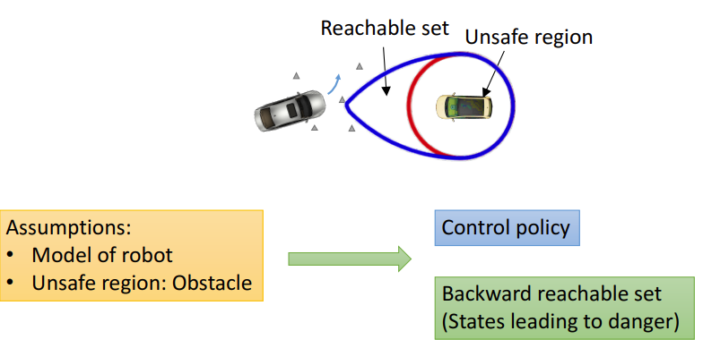
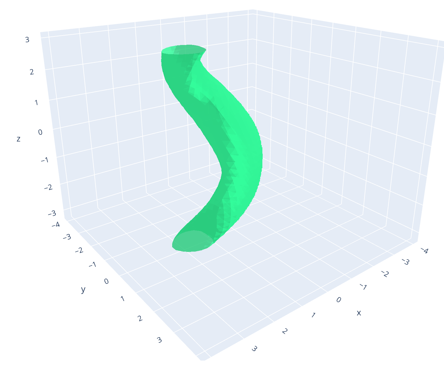
The repo contains implementation of dynamic programming based algorithms in optimal control. Specifically, the solver supports 3 main classes of algorithms: level set based algorithm for solving Hamilton-Jacobi-Issac (HJI) partial differential equation (PDE) arising in reachability analysis and differential games [1], time-to-reach (TTR) computations of dynamical systems in reachability analysis [2], and value-iterations algorithm for solving continuous state-space action-space Markov Decision Process (MDP). All these algorithms share the property of being implemented on a multidimensional grid and hence, their computational complexities increase exponentially as a function of dimension. For all the aforementioned algorithms, our toolbox allows computation up to 6 dimensions, which we think is the limit of dynammic programming on most modern personal computers.
In comparison with previous works, our toolbox strives to be both efficient in implementation while being user-friendly. This is reflected in our choice of having Python as a language for initializing problems and having python-like HeteroCL [3] language for the core algorithms implementation and dynamical systems specification. Our implementation is 7-32x faster than the Level Set Toolbox and HelperOC and 2-3x faster than BEACLS implementation in C++. Please find more details about using the repo for solving your problems in this page, and should you have any questions/problems/requests please direct the messages to Minh Bui at buiminhb@sfu.ca
Please install the following:
-
Install Anaconda (https://docs.anaconda.com/anaconda/install/linux/)
-
Create a virtual environemnt using the provided
environment.ymlconda env create -f environment.yml -
Install the
optimized_dprepositorypip install -e . -
Note: If you're on Ubuntu 20.04 or 22.04, you may have encounter an error regarding
libtinfo5. To fix, please just run this commandsudo apt install libtinfo5
- We provide a running example of solving HJI PDE in the file
examples/low_dimensional_plotting_example.py:
# STEP 1: Define grid
grid_min = np.array([-4.0, -4.0, -math.pi])
grid_max = np.array([4.0, 4.0, math.pi])
dims = 3
N = np.array([40, 40, 40])
pd=[2]
g = Grid(grid_min, grid_max, dims, N, pd)

# STEP 2: Generate initial values for grid using shape functions
center = np.zeros(dims)
radius = 1.0
ignore_dims = [2]
Initial_value_f = CylinderShape(g, ignore_dims, center, radius)

# STEP 3: Time length for computations
lookback_length = 2.0
t_step = 0.05

small_number = 1e-5
tau = np.arange(start=0, stop=lookback_length + small_number, step=t_step)

# STEP 4: User-defined System dynamics for computation
sys = DubinsCapture(uMode="max", dMode="min")

po2 = PlotOptions(do_plot=False, plot_type="3d_plot", plotDims=[0,1,2],
                  slicesCut=[])

# STEP 5: Initialize plotting option
po1 = PlotOptions(do_plot=True, plot_type="set", plotDims=[0,1,2])

# STEP 6: Call HJSolver function (BRS)
compMethod = { "TargetSetMode": "None"}
result_3 = HJSolver(sys, g, Initial_value_f, tau, compMethod, po1, saveAllTimeSteps=True)- To run the example, execute the command
python3 low_dimensional_plotting_example.py - If the parameter
do_plotis set toTrue, when initializingPlotOptions. The parametersaveAllTimeStepsis set toFalseinHJSolver, an static 3D plot will show on pop-up browser.
- If interactive 3D animation needs to be visualized, and outputs need to be saved locally
# While file needs to be saved locally, set save_fig=True and filename, recommend to set interactive_html=True for better interaction
po2 = PlotOptions(do_plot=False, plot_type="set", plotDims=[0,1,2],
                  slicesCut=[], colorscale="Bluered", save_fig=True, filename="plots/3D_0_sublevel_set.png", interactive_html=False)

# STEP 7: Visualizing output
plot_isosurface(g, result_3, po2)- For computing result higher than 6D, check
examples/examples.py - Notes: For 6 dimensions, recommended grid size is 20-30 each dimension on system with 32Gbs of DRAM.
- Create a class file in folder dynamics/ to specify your own system dynamics. Remember to import the class in your running example.
It can noticed in user_definer.py that the class DubinsCapture is imported from the folder dynamics/, where our example system dynamics.
import heterocl as hcl

class DubinsCapture:
    def __init__(self, x=[0,0,0], wMax=1.0, speed=1.0, dMax=1.0, uMode="max", dMode="min"):
        self.x = x
        (...)
        self.dMode = dMode

    def opt_ctrl(self, t, state, spat_deriv):
        """
                :param  spat_deriv: tuple of spatial derivative in all dimensions
                        state: x1, x2, x3
                        t: time
                :return: a tuple of optimal disturbances
        """

        (...)
        return (opt_w[0], in3[0], in4[0])

    def opt_dstb(self, t, state, spat_deriv):
        """
            :param spat_deriv: tuple of spatial derivative in all dimensions
                    state: x1, x2, x3
                    t: time
            :return: a tuple of optimal disturbances
        """
        (...)
        return (d1[0], d2[0], d3[0])

    def dynamics(self, t, state, uOpt, dOpt):
        (...)
return (x_dot[0], y_dot[0], theta_dot[0])- We have provided an example in
examples/TTR_example.py:
# -------------------------------- ONE-SHOT TTR COMPUTATION ---------------------------------- #
g = Grid(minBounds=np.array([-3.0, -1.0, -math.pi]), maxBounds=np.array([3.0, 4.0, math.pi]),
         dims=3, pts_each_dim=np.array([50, 50, 50]), periodicDims=[2])
# Car is trying to reach the target
my_car = DubinsCar(uMode="min")

# Initialize target set as a cylinder
targetSet = CylinderShape(g, [2], np.array([0.0, 1.0, 0.0]), 0.70)
po = PlotOptions( "3d_plot", plotDims=[0,1,2], slicesCut=[],
                  min_isosurface=lookback_length, max_isosurface=lookback_length)

# Convergence threshold
epsilon = 0.001
V_0 = TTRSolver(my_car, g, targetSet, epsilon, po)- To run the example :
python3 TTR_example.py
- solver.py: Containing python APIs to interact with the numerical solver
- dynamics/ : User's dynamical system specification
- Shapes/ShapesFunctions.py : Add-in functions for initializing different shapes/intial value functions
- computeGraphs/CustomGraphFunctions.py: Ready-to-user HeteroCL style utility functions
Please cite our paper (https://arxiv.org/abs/2204.05520) if you use the toolbox in your research:
@misc{https://doi.org/10.48550/arxiv.2204.05520,
  doi = {10.48550/ARXIV.2204.05520},
  url = {https://arxiv.org/abs/2204.05520},
  author = {Bui, Minh and Giovanis, George and Chen, Mo and Shriraman, Arrvindh},
  keywords = {Systems and Control (eess.SY), FOS: Electrical engineering, electronic engineering, information engineering, FOS: Electrical engineering, electronic engineering, information engineering},
  title = {OptimizedDP: An Efficient, User-friendly Library For Optimal Control and Dynamic Programming},
  publisher = {arXiv},
  year = {2022},
  copyright = {Creative Commons Attribution 4.0 International}
}
[1] "Hamilton–Jacobi Reachability: Some Recent Theoretical Advances and Applications in Unmanned Airspace Management" by Mo Chen and Claire J. Tomlin in Annual Review of Control, Robotics, and Autonomous Systems 2018 1:1, 333-358 pdf
[2] "One-Shot Computation of Reachable Sets for Differential Games" by Insoon Yang pdf
[3] "HeteroCL: A Multi-Paradigm Programming Infrastructure for Software-Defined Reconfigurable Computing" by Yi-Hsiang Lai pdf

