- Marco D'Antini (10603556)
- Simone Giampà (10659184)
- Gabriele Pagano (10578117)
| File | Description |
|---|---|
parameters.cfg |
configuration file for the dynamic reconfiguration of the integration method parameters |
'images' folder |
screenshots of the plots and graphs |
Control.h |
header file for the Control class |
Odometry.h |
header file for the Odometry class |
Control.cpp |
publishes the wheel velocities in [RPM] (revolutions per minute) given the robot angular and linear velocities |
Odometry.cpp |
Computation of robot odometry and robot velocities; service for changing the robot pose; dynamic reconfiguration of the integration method; callbacks for creating a new bag for the parameters estimation script |
odometry.launch |
launch file that runs the whole project |
odom.msg |
message file containing the computed odometry to be published |
record.msg |
message file containing the recorded data used for calibration |
wheels_rpm.msg |
message file containing the wheel velocities to be published (expressed in [RPM = revolutions per minute]) |
estimator.py |
Python code used for the calibration of the robot dimensions (r, l, w, N) |
set_odometry.srv |
service file containing the coordinate values to be set via the /set_odometry service |
Used to change the x, y, theta coordinates of the robot odometry at runtime. In order to set the <x, y, theta> coordinates via a service, type the following command:
rosservice call /set_odometry <new_x> <new_y> <new_theta>
Where new_x, new_y and new_theta are the new odometry pose values to be assigned
Used to set the integration method for the odometry computation to EULER or RUNGE-KUTTA approximation methods. After the nodes have been launched, it is possible to configure this ROS parameter. Dynamic reconfiguration can be done by typing:
rosrun rqt_reconfigure rqt_reconfigure
Then a window will be opened and the user can select the integration method.
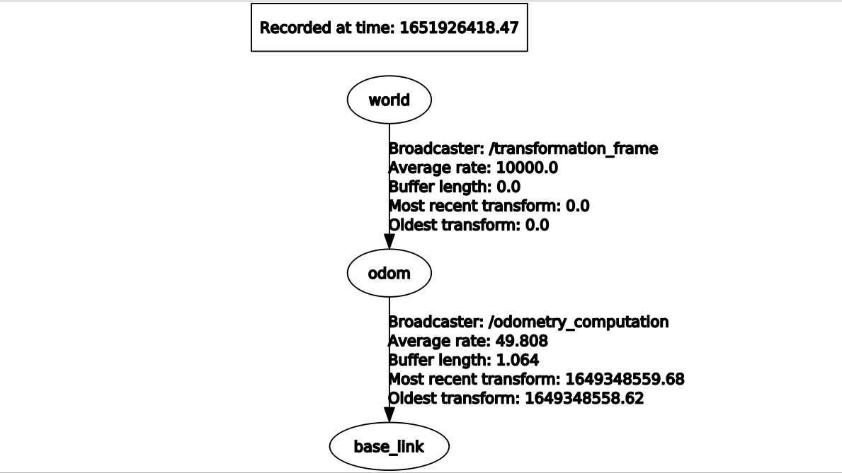
After have run the file bag1.bag, we visualized the structure of the TF tree thanks to the following command:
rosrun rqt_tf_tree rqt_tf_tree
Thus, we obtained the following:
- nav_msgs/Odometry odom: odometry published in terms of orientation (with the quaternion <x,y,z,w>) and position (with the tuple <x,y,z>)
- std_msgs/String method: method of approximation used for the odometry computation (Euler or Runge-Kutta)
- header: contains the timestamps and sequence IDs
- pose_x: x coordinate retrieved from the /robot/pose topic
- pose_y: y coordinate retrieved from the /robot/pose topic
- pose_theta: theta coordinate (expressed as euler coordinate) computed from the orientation present in the /robot/pose topic (expressed as a quaternion)
- ticks1: ticks position of the front left wheel recorded in the /wheel_states topic
- ticks2: ticks position of the front right wheel recorded in the /wheel_states topic
- ticks3: ticks position of the rear left wheel recorded in the /wheel_states topic
- ticks4: ticks position of the rear right wheel recorded in the /wheel_states topic
- header: contains the timestamps and sequence IDs
- rpm_fl: velocity of the front left wheel
- rpm_fr: velocity of the front right wheel
- rpm_rl: velocity of the rear left wheel
- rpm_rr: velocity of the rear right wheel
Each velocity is computed from the robot relative velocities, and are expressed in revolutions per minute.
- x: x coordinate to be set by the /set_odometry service
- y: y coordinate to be set by the /set_odometry service
- theta: theta coordinate to be set by the /set_odometry service
In order to start all the nodes type the following command:
roslaunch odometry_project odometry.launch
The parameters were previously optimized as they were independent, and we also created a few plots to show the error value as function of the various parameter values which we simulated. So in the images folder there are still those plots. Then we changed the structure in order to optimize the values using the ticks positions and we didn't assume anymore that the values were independent with respect to each other. With this way it is not possible anymore to create nice looking 2d or 3d plots of the error function, since it depends from multiple variables.

