The goals / steps of this project are the following:
- Perform a Histogram of Oriented Gradients (HOG) feature extraction on a labeled training set of images and train a classifier Linear SVM classifier
- Apply a color transform and append binned color features, as well as histograms of color, to your HOG feature vector.
- for those first two steps normalize your features and randomize a selection for training and testing.
- Implement a sliding-window technique and use your trained classifier to search for vehicles in images.
- Run the pipeline on a video stream (start with the test_video.mp4 and later implement on full project_video.mp4) and create a heat map of recurring detections frame by frame to reject outliers and follow detected vehicles.
- Estimate a bounding box for vehicles detected.
Note: (Code snippets taken from Udacity SD course)
The code for this step is contained in the first 12 code cells of the IPython notebook (vehicle_detection.ipnyb).
I started by reading in all the vehicle and non-vehicle images. Here is an example of one of each of the vehicle and non-vehicle classes:
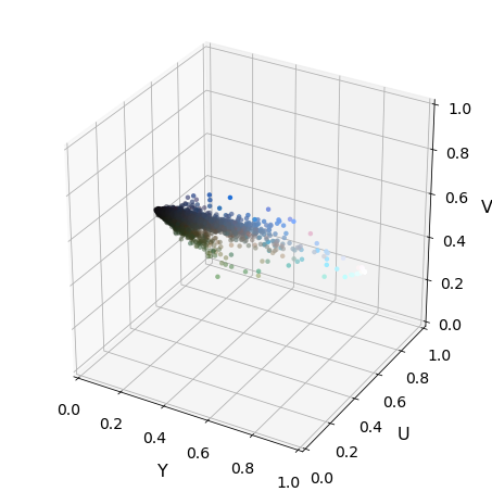
I then explored different color spaces. Different color spaces visualized in 3D space are shown below. YUV and YCrCb contain similar information. RGB, HSV, HSL have similar features for vehicle and non-vehicle images, so it is hard to create a classfier by using these color space. LUV is another good prospect but gave more error when used. Here is the visualization of the color spaces.
 Then different
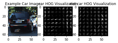
 skimage.hog() parameters (orientations, pixels_per_cell, and cells_per_block). I grabbed random images from each of the two classes and displayed them to get a feel for what the skimage.hog() output looks like.
Here is an example using the YUV color space and HOG parameters of orientations=9, pixels_per_cell=(8, 8) and cells_per_block=(2, 2):
I tried various combinations of parameters using the grid search and found that HOG channels encode most of the required features. The params gave a little more than 99% accuracy with the test. set. Hist bins and color spacial bins are not that useful features. Increasing number of orientations add to more computation and it then takes more time to create the video. Not that 2nd (last channel - V) gives NaN output when getting the HOG output if the image is from 0-1. So, I had to scale the image to 0-255 to deal with this issue.
I trained a linear SVM. The features were normalized using standard scaler from sklearn. The data was randomly shuffled and splitted into training and test sets 1/5 ratio. The code is in the 16th cell of the ipython notebook
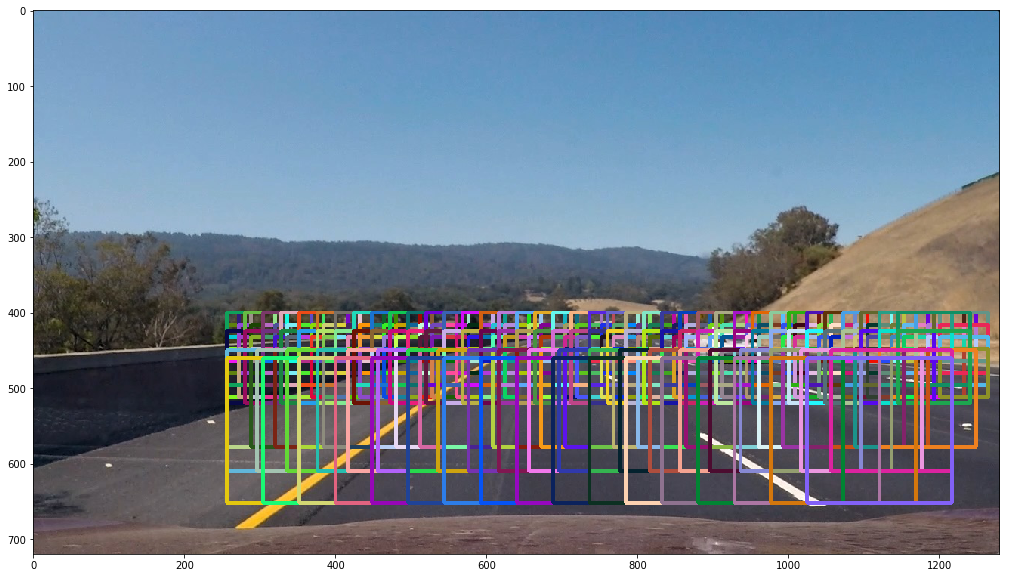
I decided to search with small windows size in around the center of the image and with larger windows size at the bottom of the image (As the cars near the camera appear to be bigger in the image). The scales of 1, 1,5, 2, 2.5 and 3 were seleted to make the pipeline robust for different scales of the car. The overlap of 0.75 was selected to make the computation faster. Then the images were converted to a heatmap, on which a threshold was applied to remove the noises. Sliding windows can be seen in the image below:
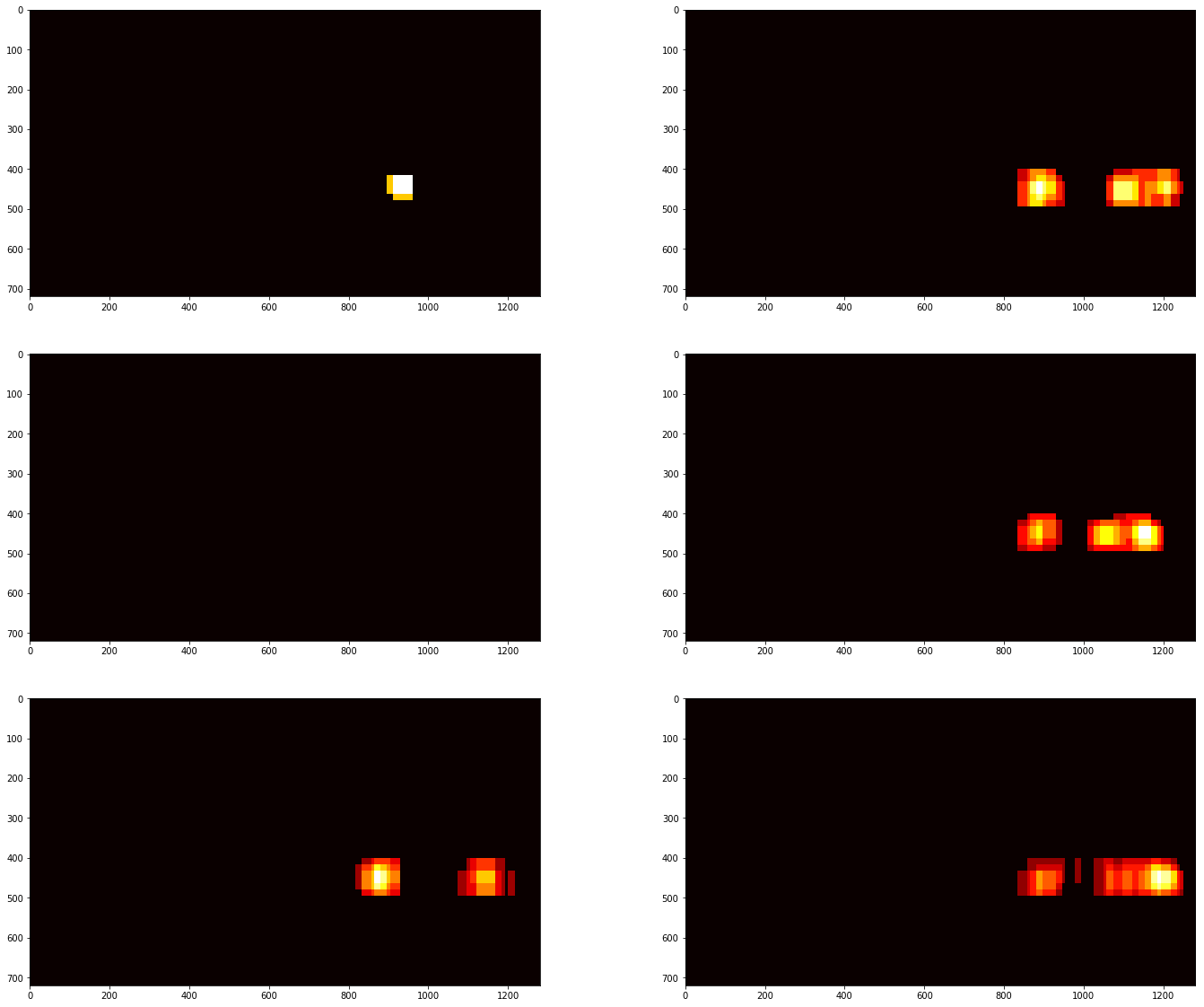
Here is the heatmap for the test images
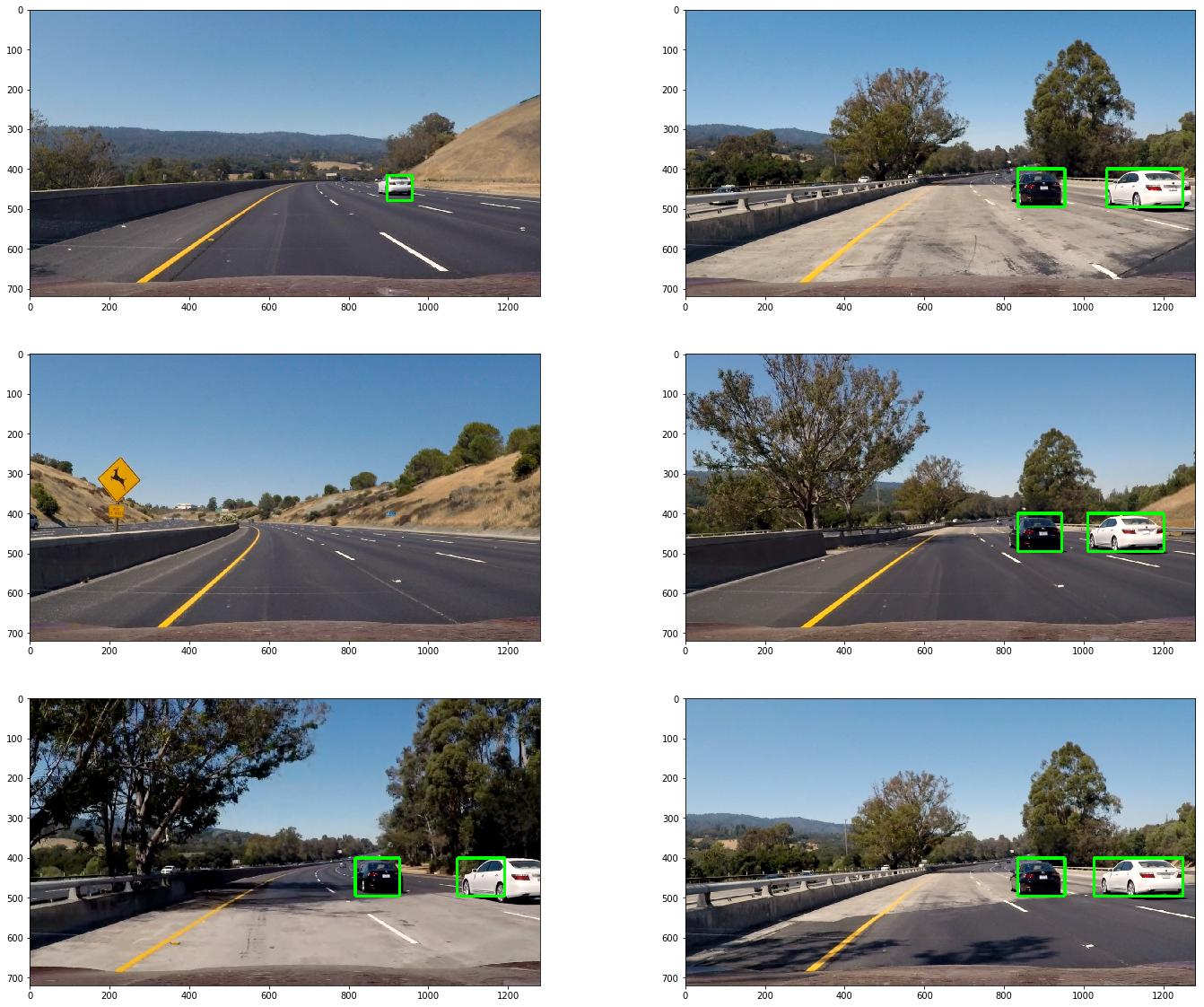
And the bounding boxes after thresholding looks like this:
Here's a link to my video result
I recorded the positions of all detections in each frame. Then after every N (5) frames I did the following:
- Created heatmap of individual frames
- Threshold heatmap of individual frames
- Combinate heatmap of all N (5) frame
- Threshold the accumulated heatmap.
- Used
scipy.ndimage.measurements.label()to identify individual blobs in the heatmap and assumed each blob corresponded to a vehicle - Constructed bounding boxes to cover the area of each blob detected.
All the frames are bboxes from the individual frames are inserted into queue and this way bboxes of last 5 frames are retained. This make the pipeline more robust.
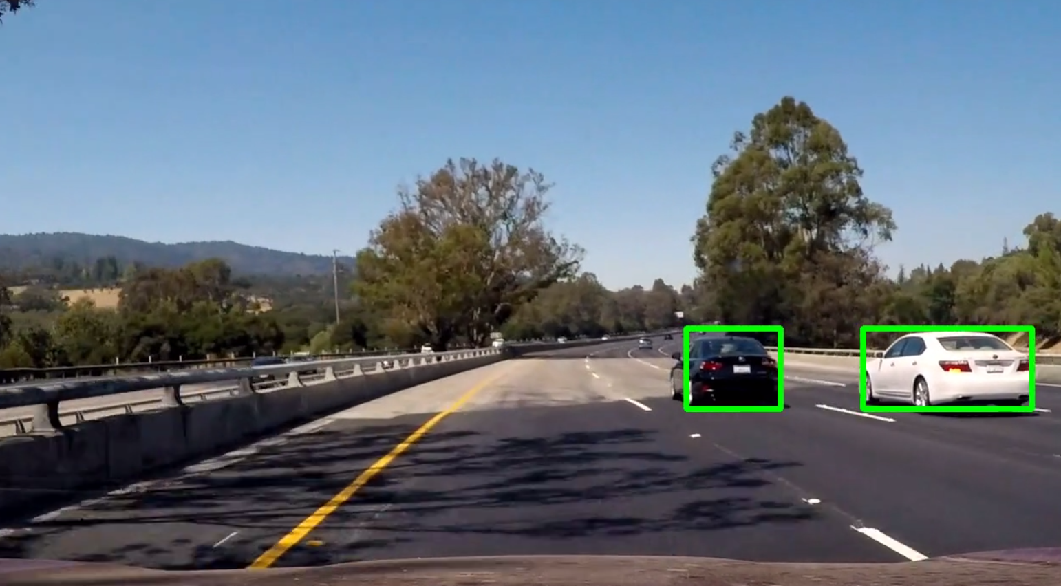
Here's an example result showing the heatmap from a series of frames of video, the result of scipy.ndimage.measurements.label() and the bounding boxes then overlaid on the last frame of video:
1. Briefly discuss any problems / issues you faced in your implementation of this project. Where will your pipeline likely fail? What could you do to make it more robust?
Problems faces:
- HOG gives NaN values for V (of YUV) channel. Need to scale images to 0-255 for this.
- Tuning the hyperparameters is very uinteresting and time consuming
Failures:
- Different lighting conditions like night or video from different weather conditions
- Tracking is not robust
- Doesn't work for small cars
Next Steps to improve:
- Use kalman filter for tracking
- Use CNN for detection


