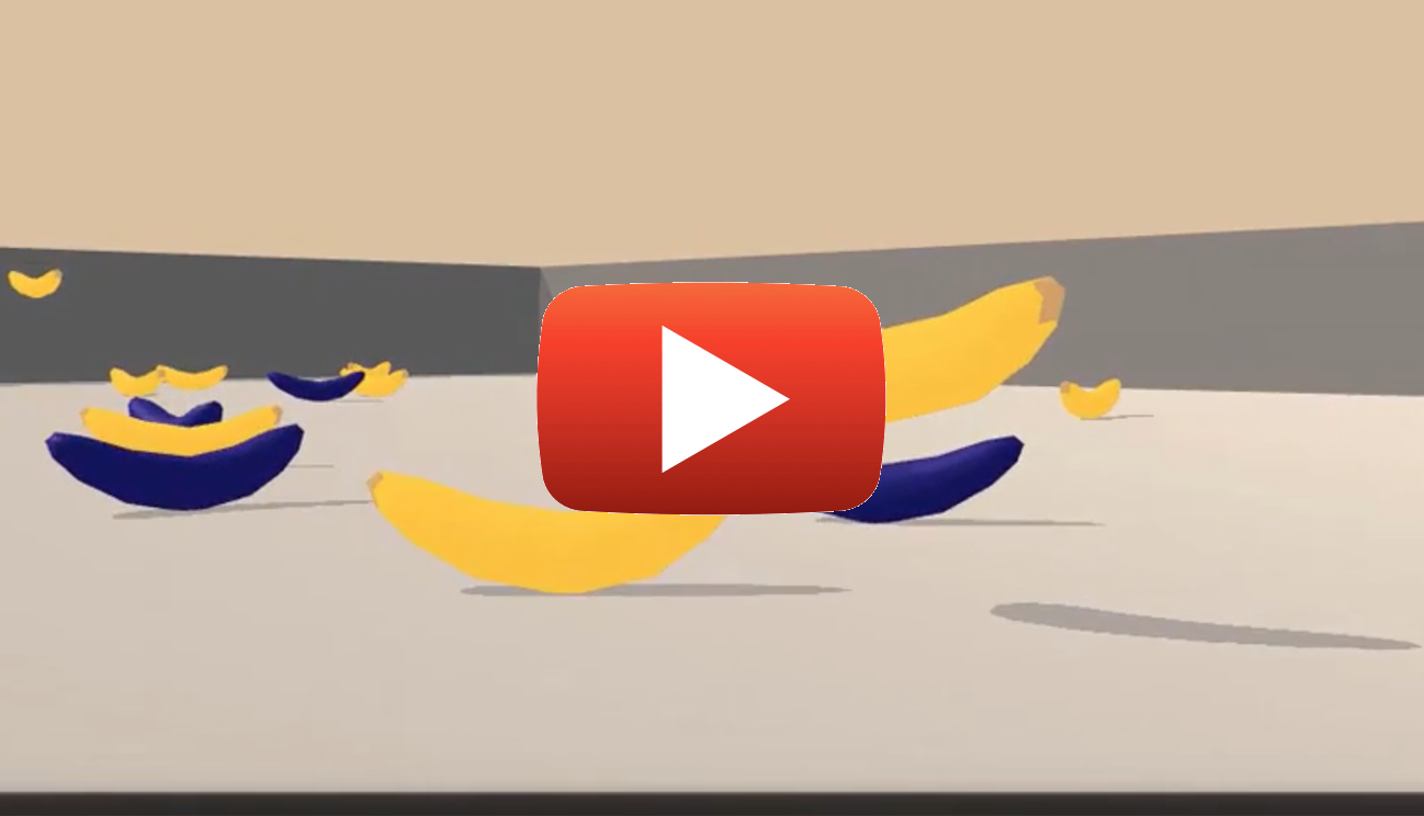
For this project, I had to train an agent to navigate (and collect bananas!) in a large, square world.
A reward of +1 is provided for collecting a yellow banana, and a reward of -1 is provided for collecting a blue banana. Thus, the goal of the agent is to collect as many yellow bananas as possible while avoiding blue bananas.
The state space has 37 dimensions and contains the agent's velocity, along with ray-based perception of objects around agent's forward direction. Given this information, the agent has to learn how to best select actions. Four discrete actions are available, corresponding to:
0- move forward.1- move backward.2- turn left.3- turn right.
The task is episodic, and in order to solve the environment, the agent must get an average score of +13 over 100 consecutive episodes.
To see if the agent interacts with the simulated environment, it was tested by performing random actions.
env_info = env.reset(train_mode=False)[brain_name] # reset the environment
state = env_info.vector_observations[0]            # get the current state
score = 0                                          # initialize the score
while True:
    action = np.random.randint(action_size)        # select an action
    env_info = env.step(action)[brain_name]        # send the action to the environment
    next_state = env_info.vector_observations[0]   # get the next state
    reward = env_info.rewards[0]                   # get the reward
    done = env_info.local_done[0]                  # see if episode has finished
    score += reward                                # update the score
    state = next_state                             # roll over the state to next time step
    if done:                                       # exit loop if episode finished
        break

print("Score: {}".format(score))
Running this agent a few times resulted in scores from -2 to 2. Obviously randomness doens't help to reach a score of +13.
Agents use a policy to decide which actions to take next within the environment. The primary goal of the learning algorithm is to find an optimal policy—i.e., a policy which maximizes the returned reward for the agent. Since the effects of possible actions aren't known in advance, the optimal policy must be discovered by interacting with the environment and recording observations. Therefore, the agent "learns" the policy through the principle of "carrot and stick" that iteratively maps various environment states to the actions that yield the highest reward. This type of algorithm is called Q-Learning.
The general approach to generate the Q-Learning algorithm is to implement the basic algorithm structure, add different components and run various tests with changing hyperparameters to yield the best results.
In the following sections, each component of the algorithm is described in detail.
To discover an optimal policy, a Q-function is used. The Q-function calculates the expected reward R for all possible actions A in all possible states S.
We can then define our optimal policy π* as the action that maximizes the Q-function for a given state across all possible states. The optimal Q-function Q*(s,a) maximizes the total expected reward for an agent starting in state s and choosing action a, then following the optimal policy for each subsequent state.
In order to discount returns at future time steps, the Q-function can be expanded to include the hyperparameter gamma γ.
The agent has to choose between performing an action based on already observed ergo known Q-values or try a completly new action with the chance of earning a higher reward and discovering new strategies. This is called the exploration vs. exploitation dilemma.
To solve this, an 𝛆-greedy algorithm was implemented. This algorithm allows the agent to systematically manage the exploration vs. exploitation trade-off. The agent "explores" by picking a random action with some probability epsilon 𝛜. However, the agent continues to "exploit" its knowledge of the environment by choosing actions based on the policy with probability (1-𝛜).
Furthermore, the value of epsilon is purposely decayed over time, so that the agent favors exploration during its initial interactions with the environment, but increasingly favors exploitation as it gains more experience. The starting and ending values for epsilon, and the rate at which it decays are three hyperparameters that are later tuned during experimentation.
You can find the 𝛆-greedy logic implemented as part of the agent.act() method here in agent.py of the source code.
With Deep Q-Learning, a deep neural network is used to approximate the Q-function. Given a network F, finding an optimal policy is a matter of finding the best weights w such that F(s,a,w) ≈ Q(s,a).
The neural network architecture used for this project can be found here in the model.py file of the source code. The network contains three fully connected layers with 64, 64, and 4 nodes respectively.
As for the network inputs, rather than feeding-in sequential batches of experience tuples, random samples from a history of experiences are used to reduce correlation between the tuples. This approach is called Experience Replay.
Experience replay allows the RL agent to learn from past experience.
Each experience is stored in a replay buffer as the agent interacts with the environment. The replay buffer contains a collection of experience tuples with the state, action, reward, and next state (s, a, r, s'). The agent then samples from this buffer as part of the learning step. Experiences are sampled randomly, so that the data is uncorrelated. This prevents action values from oscillating or diverging catastrophically, since a naive Q-learning algorithm could otherwise become biased by correlations between sequential experience tuples.
Also, experience replay improves learning through repetition. By doing multiple passes over the data, our agent has multiple opportunities to learn from a single experience tuple. This is particularly useful for state-action pairs that occur infrequently within the environment.
The implementation of the replay buffer can be found here in the agent.py file of the source code.
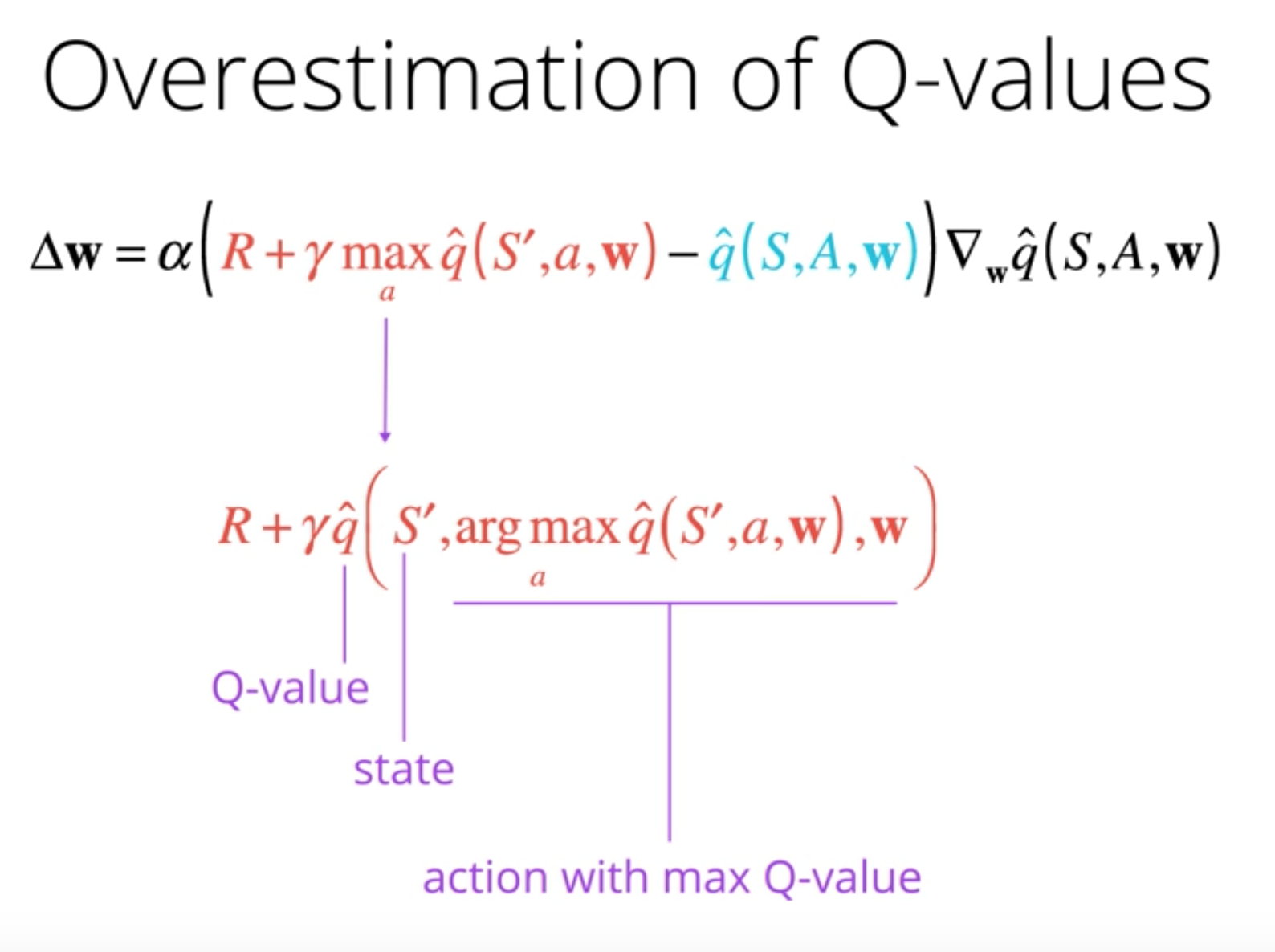
One issue with Deep Q-Networks is the possible overestimation of Q-values. The accuracy of the Q-values depends on which actions have been tried and which states have been explored. If the agent hasn't gathered enough experiences, the Q-function will end up selecting the maximum value from a noisy set of reward estimates. Early in the learning phase, this can cause the algorithm to propagate incidentally high rewards that were obtained by chance (exploding Q-values). This could also result in fluctuating Q-values later in the process.
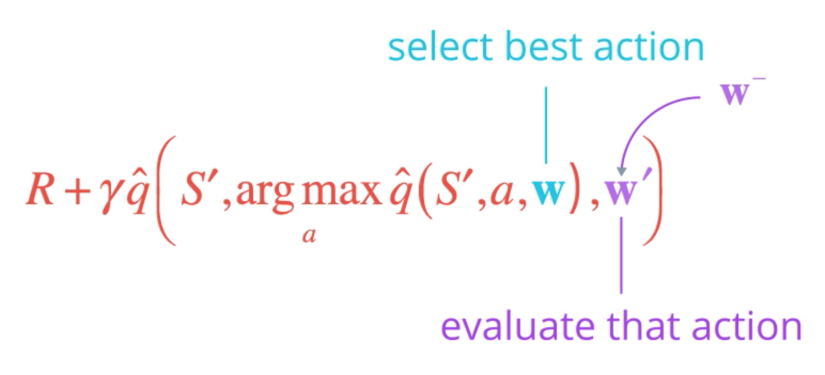
We can address this issue using Double Q-Learning, where one set of parameters w is used to select the best action, and another set of parameters w' is used to evaluate that action.
The DDQN implementation can be found here in the agent.py file of the source code.
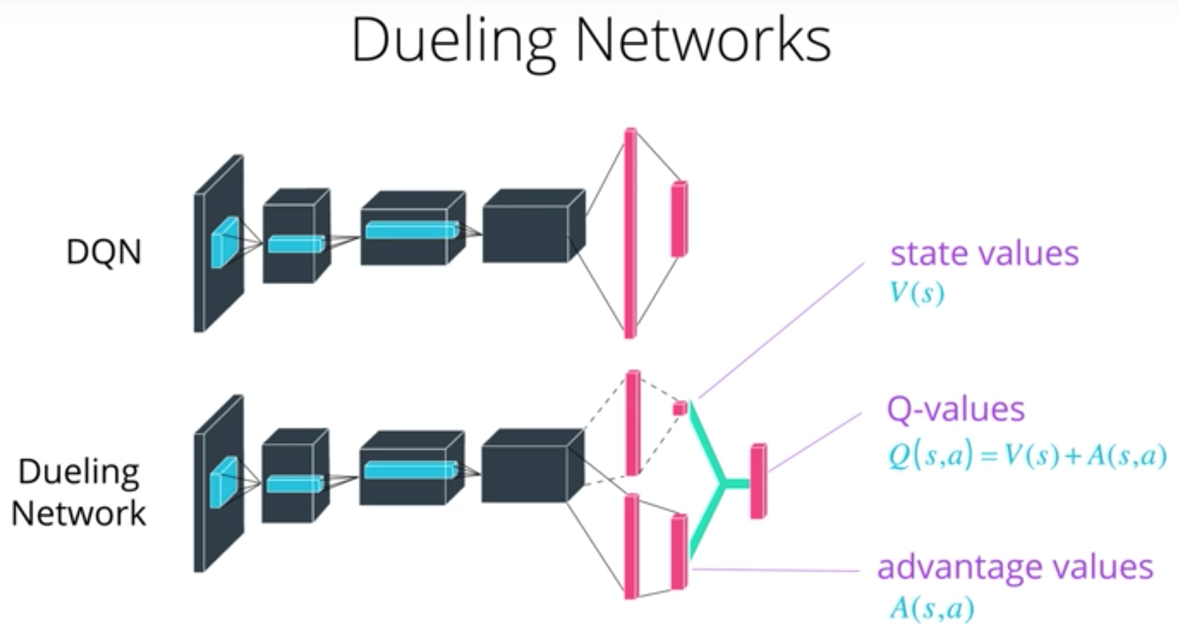
Dueling networks utilize two streams: one that estimates the state value function V(s), and another that estimates the advantage for each action A(s,a). These two values are then combined to obtain the desired Q-values.
The reasoning behind this approach is that state values don't change much across actions, so it makes sense to estimate them directly. However, we still want to measure the impact that individual actions have in each state, hence the need for the advantage function.
The dueling agents are implemented within the fully connected layers here in the model.py file of the source code.
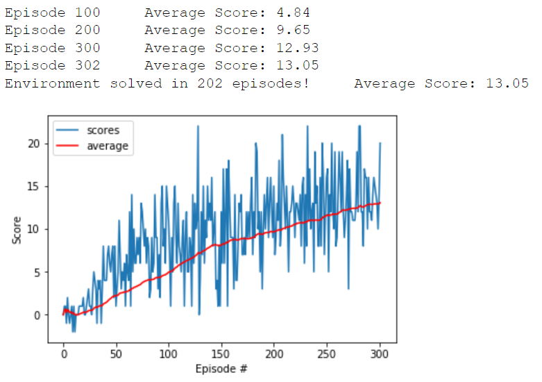
The best performing agents were able to solve the environment in 200-250 episodes. While this set of agents included ones that utilized Double DQN and Dueling DQN, at the end, the top performing agent was a simple DQN with replay buffer.
The complete set of results and steps can be found in this notebook.
Tommy Tracey, a former Udacity student loaded a video up to Youtube: here It is a video showing the agent's progress as it goes from randomly selecting actions to learning a policy that maximizes rewards.
- Test the replay buffer — Implement a way to enable/disable the replay buffer. As mentioned before, all agents utilized the replay buffer. Therefore, the test results don't measure the impact the replay buffer has on performance.
- Add prioritized experience replay — Rather than selecting experience tuples randomly, prioritized replay selects experiences based on a priority value that is correlated with the magnitude of error. This can improve learning by increasing the probability that rare and important experience vectors are sampled.
- Use a CNN with more layers and more nodes
-
Download the environment from one of the links below. You need only select the environment that matches your operating system:
- Linux: click here
- Mac OSX: click here
- Windows (32-bit): click here
- Windows (64-bit): click here
(For Windows users) Check out this link if you need help with determining if your computer is running a 32-bit version or 64-bit version of the Windows operating system.
(For AWS) If you'd like to train the agent on AWS (and have not enabled a virtual screen), then please use this link to obtain the environment.
-
Place the file in the DRLND GitHub repository, in the
p1_navigation/folder, and unzip (or decompress) the file.
Follow the instructions in Navigation.ipynb to get started with training your own agent!
After you have successfully completed the project, if you're looking for an additional challenge, you have come to the right place! In the project, your agent learned from information such as its velocity, along with ray-based perception of objects around its forward direction. A more challenging task would be to learn directly from pixels!
To solve this harder task, you'll need to download a new Unity environment. This environment is almost identical to the project environment, where the only difference is that the state is an 84 x 84 RGB image, corresponding to the agent's first-person view. (Note: Udacity students should not submit a project with this new environment.)
You need only select the environment that matches your operating system:
- Linux: click here
- Mac OSX: click here
- Windows (32-bit): click here
- Windows (64-bit): click here
Then, place the file in the p1_navigation/ folder in the DRLND GitHub repository, and unzip (or decompress) the file. Next, open Navigation_Pixels.ipynb and follow the instructions to learn how to use the Python API to control the agent.
(For AWS) If you'd like to train the agent on AWS, you must follow the instructions to set up X Server, and then download the environment for the Linux operating system above.


