This package estimates the calibration parameters that transforms the camera frame (parent) into the lidar frame (child). We aim to simplify the calibration process by optimising the pose selection process to take away the tedious trial-and-error of having to re-calibrate with different poses until a good calibration is found. We seek to obtain calibration parameters as an estimate with uncertainty that fits the entire scene instead of solely fitting the target, which many existing works struggle with. Our proposed approach overcomes the limitations of existing target-based calibration methods, namely from user error and overfitting of the target. For more details, please take a look at our paper.
We also provide a video tutorial for this package which you can follow alongside this readme.
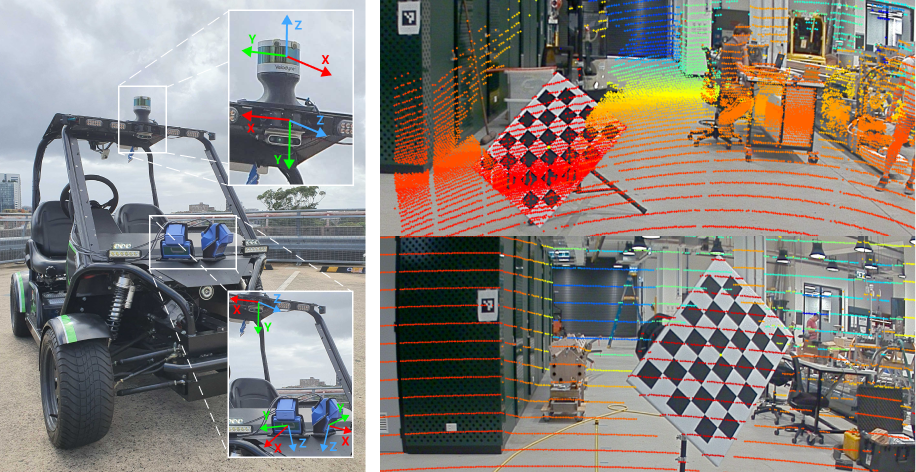
Left: Our sensor setup at the Australian Centre for Field Robotics (ACFR). Right: Calibration results of this package with an Nvidia gmsl camera to both Baraja Spectrum-Scan™ (top) and Velodyne VLP-16 (bottom). The projection of Baraja Spectrum-Scan™ has some ground points (yellow) on the chessboard due to the difference in perspective of camera and lidar.
This package has only been tested in ROS Melodic.
- Clone the repository in your
catkin_ws/src/folder
git clone -c http.sslverify=false https://gitlab.acfr.usyd.edu.au/its/cam_lidar_calibration.git
- Download ros and python dependencies
sudo apt update && sudo apt-get install -y ros-melodic-pcl-conversions ros-melodic-pcl-ros ros-melodic-tf2-sensor-msgs
pip install pandas scipy
- Build the package and source the
setup.bashorsetup.zshfile.
catkin build cam_lidar_calibration
source ~/catkin_ws/devel/setup.bash
- Clone the repository in your
catkin_ws/src/folder
git clone -c http.sslverify=false https://gitlab.acfr.usyd.edu.au/its/cam_lidar_calibration.git
- Run the docker image (which will be pulled dockerhub). If your computer has a Nvidia GPU, set the cuda flag
--cuda on. If you do not have one, set--cuda off.
cd cam_lidar_calibration/docker
./run.sh --cuda on
Once you run this script, the docker container will run and immediately build the catkin workspace and source the setup.bash file. When this is done, you can move on to the Quick start section.
If you'd like to build the image from scratch, a build.sh script is also provided.
Note: If using docker, the ./run.sh mounts your local cam_lidar_calibration folder to /catkin_ws/src/cam_lidar_calibration inside the container. When running the calibration, this would create csv files inside the container under root ownership which is not ideal. However the workaround is to use the following command outside the docker image, which would change ownership of all files in your current folder to be the same as your $USER and $GROUP in the local environment.
sudo chown $USER:$GROUP *
You can verify that this repository runs sucessfully by running this package on our provided quick-start data. If you are using docker, these instructions should be run inside the container.
1. Run the calibration process
This first step takes the saved poses, computes the best sets with the lowest VOQ score.
roslaunch cam_lidar_calibration run_optimiser.launch import_samples:=true
After calibration, the output is saved in the same directory as the imported samples. For this quickstart example, the output is saved in cam_lidar_calibration/data/vlp/.
2. Obtain and assess calibration results
This step gives the estimated calibration parameters by taking a filtered mean of the best sets, and displaying the gaussian fitted histogram of estimated parameters. Additionally, we provide an assessment of the calibration results by computing the reprojection error over all provided data samples and a visualisation (if specified).
To obtain and assess the calibration output, provide the absolute path of the csv output file generated in the first step. The example below uses pre-computed calibration results. You can replace this with your newly generated results in step 1 if you wish. You should see a terminal output with the reprojection errors, along with a gaussian-fitted histogram and a visualisation.
roslaunch cam_lidar_calibration assess_results.launch csv:="$(rospack find cam_lidar_calibration)/data/vlp/calibration_quickstart.csv" visualise:=true
That's it! If this quick start worked successfully, you can begin using this tool for your own data. If not, please create an issue and we'll aim to resolve it promptly.
To use this package with your own data, ensure that your bag file has the following topics:
- Lidar: 3D pointcloud of point type XYZIR, published as sensor_msgs::PointCloud2. This package relies on the ring value and so if you don't have that, you need to modify your lidar driver to use this package.
- Monocular camera: an image published as sensor_msgs::Image and the corresponding meta-information topic (sensor_msgs::CameraInfo).
All data and output files will be saved in the cam_lidar_calibration/data/YYYY-MM-DD_HH-MM-SS/ folder.
- Prepare a rectangular chessboard printout. The chessboard print used in the paper is an A1 (594 x 841mm) with 95mm squares and 7x5 inner vertices (not the same as the number of grid squares), downloaded from https://markhedleyjones.com/projects/calibration-checkerboard-collection
- Firmly attach the chessboard on a rigid, opaque, and rectangular board such that both their centres align (as best as possible) and their edges remain parallel to one another.
- Choose a suitable stand that can mount the target with little to no protruding elements from the board's edges.
- Rotate the chessboard such that it is in the shape of a diamond (at an angle of 45° with respect to the ground) and mount it on a stand.
In the image below, we show two chessboards rigs that we've used with this package.
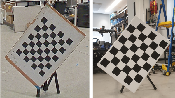
Left: chessboard with 8x6 inner vertices and 65mm squares. Right: chessboard with 7x5 inner vertices and 95mm squares.
The following explains the fields in /cfg/params.yaml
1. Specify the names of your lidar and camera topics. For example, in our case it is:
camera_topic: "/gmsl/A0/image_color"
camera_info: "/gmsl/A0/camera_info"
lidar_topic: "/velodyne/front/points"
2. (optional) Specify the default bounds of the pointcloud filtering. If you are unsure, feel free to skip this step.
3. Input the details about the chessboard target you prepared:
- pattern_size: these are the inner vertices of the chessboard (not the number of squares; see our chessboards in Section 2.1)
- square_length (mm): the length of a chessboard square.
- board_dimension (mm): width and height of the backing board that the chessboard print is mounted on.
- translation_error: the offset of the chessboard centre from the centre of the backing board (see illustration below).
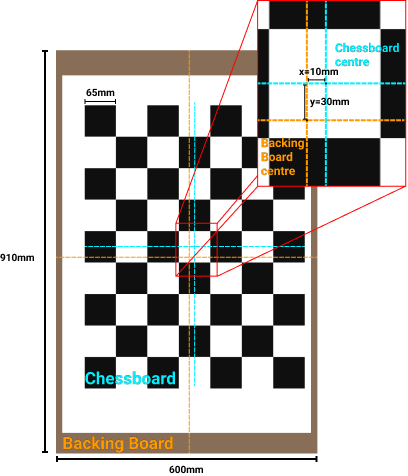
Example: In this example, the offset is x=10mm, y=30mm, board dimensions are 910x650mm with square lengths of 65mm and pattern size of 8x6 (HxW).
Run the calibration package with the import_samples flag set to false. An rviz window and rqt dynamic reconfigure window should open. If you're using a docker container and RViz does not open, try setting the cuda flag to the opposite of what you used.
roslaunch cam_lidar_calibration run_optimiser.launch import_samples:=false
This process can be done online or offline. If you are offline, make sure to play the rosbag using --pause flag so that rviz can get the /tf topics e.g. rosbag play --pause mybag.bag. If you are running a docker container, you can run the bag file on a separate terminal window outside the docker container.
Make sure to change the image topic to your camera image topic in order to see the video feed. This can be done by editing line 62 of cam_lidar_calibration.rviz or open rviz->panels->display, and change the field that is currently /gmsl/A0/image_color.
Using the rqt_reconfigure window, modify the values of the x,y and z axes limits to such that it only shows the chessboard. If chessboard is not fully isolated, it may affect the plane-fitting of the chessboard and also lead to high board dimension errors.

Left: Unfiltered pointcloud. Right: isolated chessboard pointcloud after setting the values in the rqt_reconfigure. For each chessboard pose, depending on your lidar, you might have to continually tweak the rqt_reconfigure values.
Place the chessboard facing the sensor pair and click the capture button. Make sure that the chessboard is correctly outlined with a low board dimension error. If it isn't, then discard and click capture again (or move the board and capture again).
Board errors (in the terminal window): Try to get a board dimension error as close to zero as possible (errors less than 30mm are acceptable). If the board error is too high, then try again in a different position or see below for potential fixes.
-
High board errors can be caused by the chessboard being too close or too far from the lidar. So we recommend moving it a bit closer/further.
-
Low resolution lidars may struggle to capture boards with low error if there are not enough points on the board. For example, for the VLP-16, we require at least 7 rings on the board for a decent capture.
-
If the chessboard is consistently under or overestimated with the same amount of board error, then it could be that the lidar's internal distance estimation is not properly calibrated. Lidars often have a range error of around +/-30mm and this is inconsistent at different ranges. We've provided a param in the
run_optimiser.launchfile that allows you to apply an offset to this distance estimation. Try to set the offset such that you get the lowest average error for your data (you might need to re-capture a couple times to figure this value). For our VLP-16 we had to setdistance_offset_mm=-30. This should be permanently set in the lidar driver once you've finished calibrating.
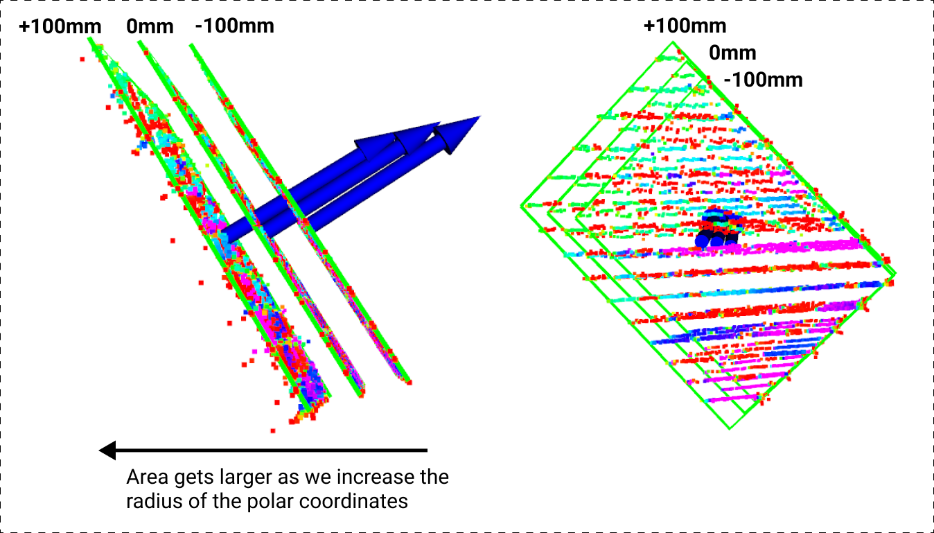
In the left image above, we show the same pose at 3 different distance offsets. We add a distance offset by converting the cartesian (xyz) coordinates to polar (r, theta) and add a distance offset to the radius r. When we do this, you can think of it like extending/reducing the radius of a circle. Every shape in that new coordinate system is hence enlarged/shrunk. Increasing the distance offset value increases the chessboard area (+100mm is the largest). The right image is the same as the left, just with a different perspective to show that the increase is in both height and width of the chessboard.
Number and variation of poses: We recommend that you capture at least 20 poses (more is better) with at least a 1-2m distance range (from lidar centre) between closest and farthest poses. Below lists some guidelines.
-
Spread the poses out in the calibration range, covering the width of the image field of view. For our specific VLP-16 and Baraja Spectrum Scan lidars, we had a range of 1.7m - 4m and 2.1m - 5m respectively.
-
Have variation in the yaw and pitch of the board as best as you can. This is explained in the following image.

For the bad poses (left), the normals of the board align such that their tips draw out a line and they are all in the same position, thereby giving a greater chance of overfitting the chessboard at that position. For the good poses (right), we see variation in the board orientation and positioning.
When all poses have been captured, click the optimise button. Note that if you do not click this button, the poses will not be properly saved.
The poses are saved (png, pcd, poses.csv) in the ($cam_lidar_calibration)/data/YYYY-MM-DD_HH-MM-SS/ folder for the reprojection assessment phase (and also if you wish to re-calibrate with the same data). The optimisation process will generate an output file calibration_YYYY-MM-DD_HH-MM-SS.csv in the same folder which stores the results of the best sets.
After you obtain the calibration csv output file, copy-paste the absolute path of the calibration output file after csv:= in the command below with double quotation marks. A histogram with a gaussian fitting should appear. You can choose to visualise a sample if you set the visualise flag. If you wish to visualise a different sample, you can change the particular sample in the assess_results.launch file. The reprojection results are shown in the terminal window.
The final estimated calibration parameters can be found in the terminal window or taken from the histogram plots.
roslaunch cam_lidar_calibration assess_results.launch csv:="$(rospack find cam_lidar_calibration)/data/vlp/calibration_quickstart.csv" visualise:=true
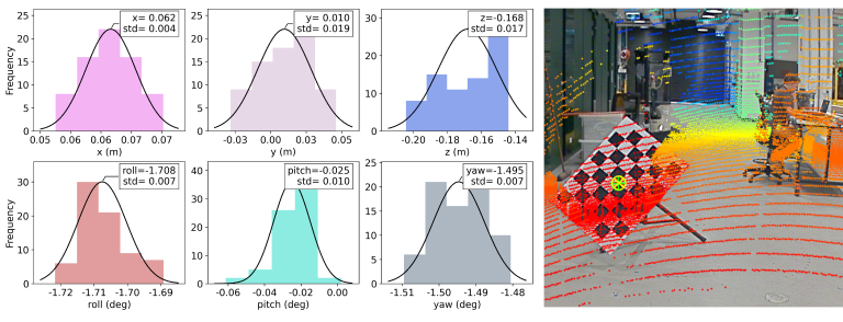
Output of our calibration pipeline shows a histogram with a gaussian fit and a visualisation of the calibration results with reprojection error.
The baseline calibration algorithm was from Verma, 2019. You can find their paper, and their publicly available code.
Please cite our work if this package helps with your research.
@article{tsai2021optimising,
  title={Optimising the selection of samples for robust lidar camera calibration},
  author={Tsai, Darren and Worrall, Stewart and Shan, Mao and Lohr, Anton and Nebot, Eduardo},
  journal={arXiv preprint arXiv:2103.12287},
  year={2021}
}