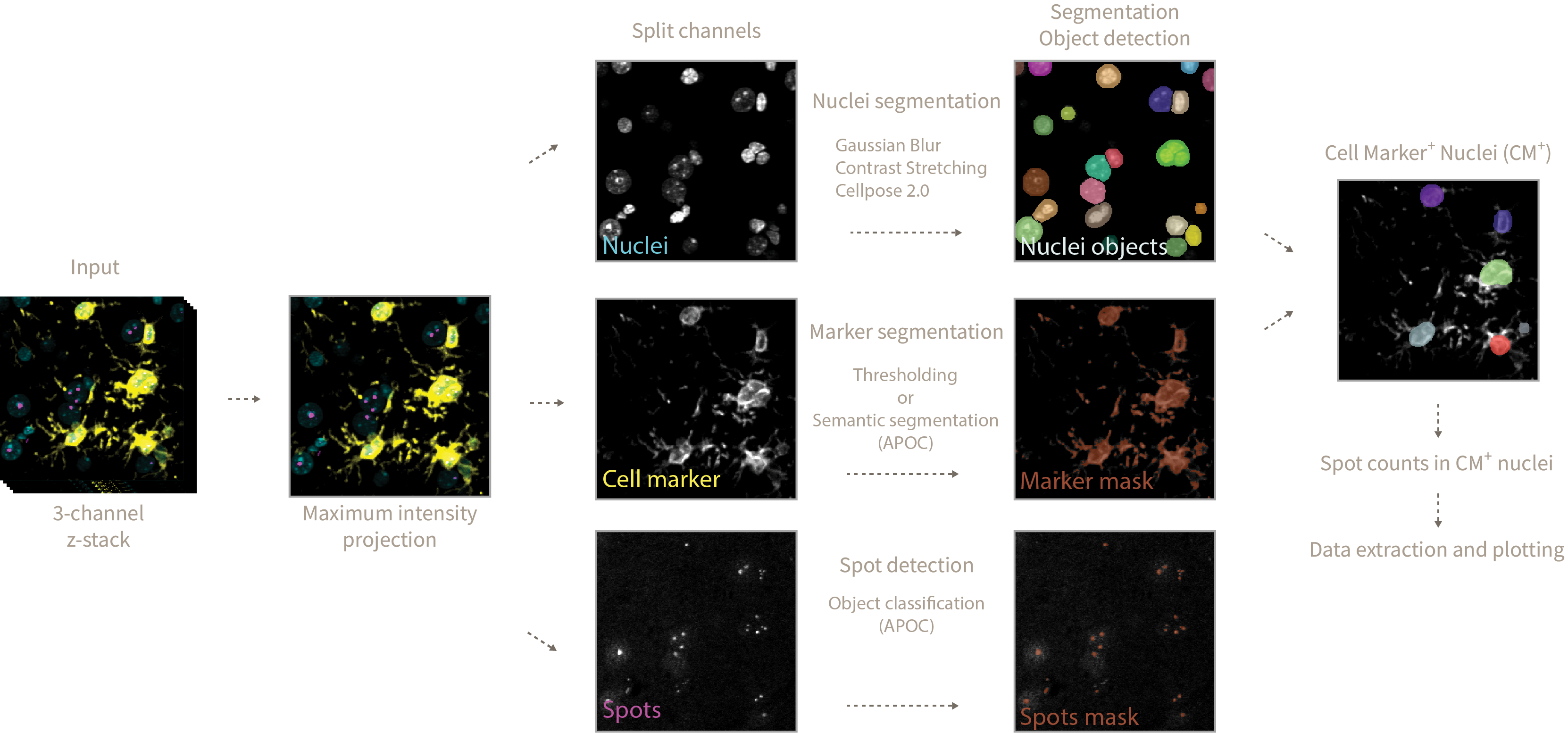
This repository provides tools in the form of interactive Jupyter notebooks to count spots inside nuclei of cell marker positive and total cells. As an example we will be counting DNA damage foci inside microglia and astrocyte marker positive cells.
-
Contact Me to obtain a fresh working S3 bucket pre-signed link.
-
Paste the link inside
0_data_download.ipynbnotebook afterpresigned_url. -
Run the notebook to download and extract the data.
-
Create a raw_data directory inside the microglia_dna_damage folder to store all of your acquired images. In our case .lsm files acquired with a Zeiss microscope. This particular tools works with 3-channel images but is easy to adapt to multiple channels.
-
(Optional) Train your own Object and Pixel (semantic) APOC classifiers to detect spots and cell marker as shown in
0_train_dna_damage_segmenter.ipynband0_train_glia_semantic_classifier.ipynb. An example of how to do that using Napari-Assistant can be found here. -
Open
1_image_analysis.ipynband define the analysis parameters. Here's an explanation of what each parameter means and does during the analysis pipeline:
- Gaussian smoothing blurs the input nuclei image so later on the Cellpose algorithm does not focus in bright spots inside the nuclei as separate objects. The amount of blurring/smoothing can be controlled by the
gaussian_sigmaparameter (default = 1).
The higher the gaussian_sigma values the increased chance of close sitting nuclei being detected as a single entity during Cellpose segmentation (see bright green nuclei below, gaussian_sigma = 6). On the other hand very low gaussian_sigma can result in incorrect segmentations or loss of nuclei entities. You will have to manually adjust this value according to your images.
-
After gaussian smoothing a normalization step of contrast stretching is applied so Cellpose segmentation does not focus in dimmer vs more intense nuclei and misses detection of some.
-
During Cellpose 2.0 nuclei segmentation you can define the
cellpose_nuclei_diametervalues. This value corresponds to the diameter in pixels of the nuclei present in your image. Helps Cellpose adjust nuclei mask predictions. -
After nuclei prediction and using .cle functions, we dilate nuclei labels to make sure the spots we want to quantify are sitting inside or touching the nuclei mask. You can define the amount of dilation by modifying the
dilation_radius_nucleivalue. -
Finally a nuclei label erosion of radius 1 is performed to avoid merging touching nuclei objects upon eventual binarization steps.
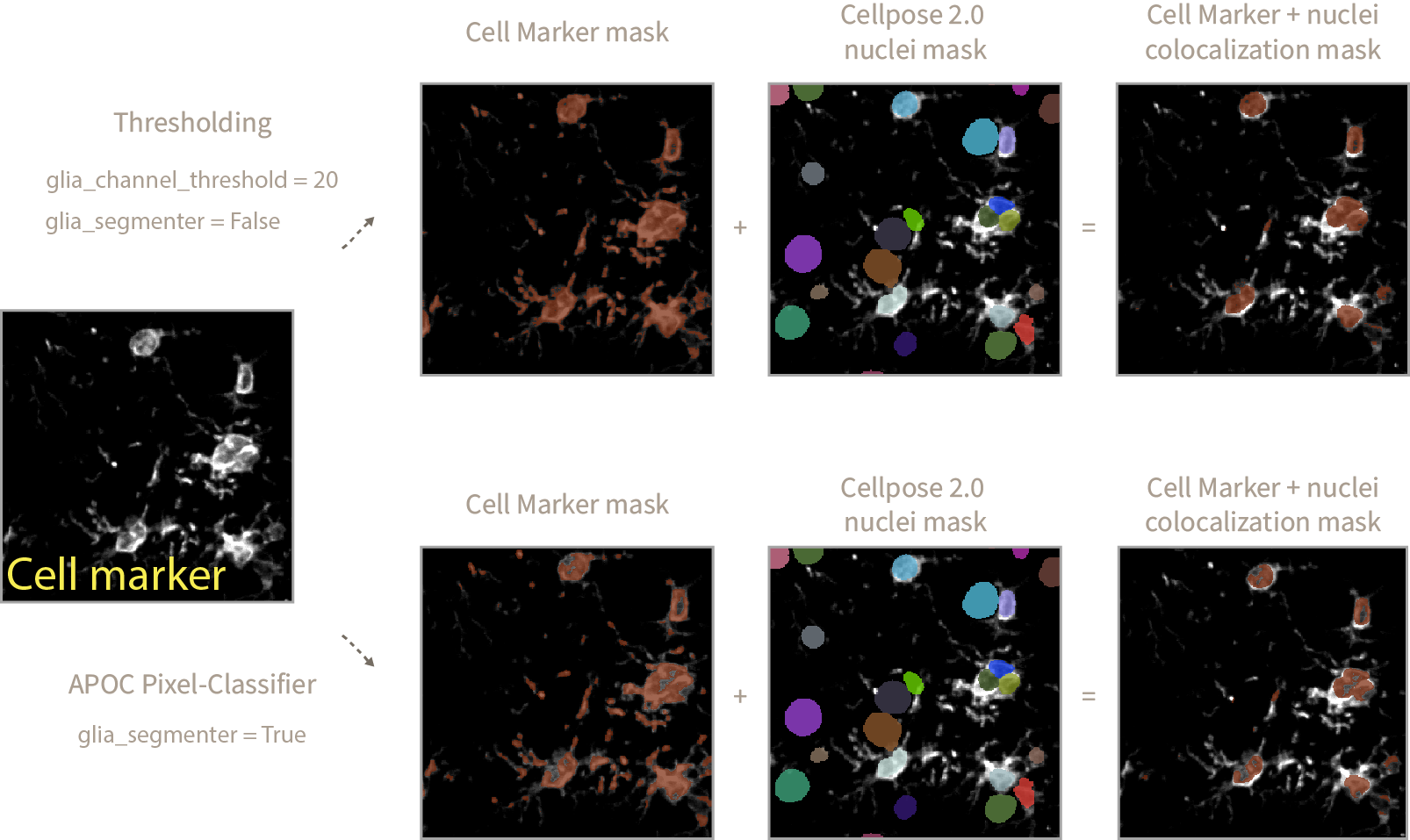
- In order to define the cell marker mask you can follow two approaches:
-
A simple thresholding approach, where any pixel above a threshold value (
glia_channel_threshold) is considered as positive cell marker signal. This approach works well if you have a clear staining with minimum background and not much variation of intensities across samples. -
A pretrained APOC-based pixel-classifier that defines what is cell marker signal and what is background. This approach works well to generalize what is cell marker signal across samples with varying levels of intensities and noise. You can train your own APOC Pixel Classifier using
0_train_glia_semantic_classifier.ipynb.
-
To use the thresholding approach define the pixel value above which any signal is considered as cell marker set
glia_channel_thresholdto your desired value and setglia_segmenter = False. -
Alternatively, set
glia_segmenter = Trueand use the pixel-classifier. Take into account that the pixel-classifier might not be as accurate (it is designed to generalize) as the thresholding method and you will need to adjust theglia_nuclei_colocalization_erosionvalue (see next steps).
-
Once you have decided on a method for cell marker segmentation you would have obtained a Cell Marker + nuclei colocalization mask defining the areas of the image where the cell marker signal is sitting on top of a nucleus.
-
In the case of microglia and astrocytic cells (our example) there are cell protrusions that might sit on top of a nucleus that does not correspond to a Cell Marker positive cell (since our input image is a stack from multiple planes that is flattened via maximum intensity projection). In order to get rid of those unwanted regions we perform an erosion of the colocalization mask. The erosion extent is defined by the
glia_nuclei_colocalization_erosionvariable. The higher the value, the stricter the conditions to consider a nucleus as CM+. Too high values will result in the complete absence of CM+ nuclei. -
Once the erosion operation is complete we check which Cellpose 2.0 detected nuclei objects sit on top of the eroded colocalization mask and mark those as CM+ nuclei. Afterwards we perform the same nuclei dilation and erosion steps defined in the Nuclei segmentation section.
-
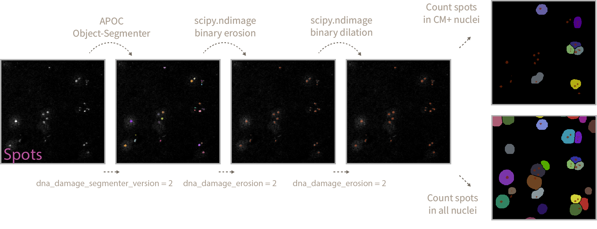
The final step in the analysis involves the detection of spots (in this example DNA damage foci) using a pretrained APOC-based object-segmenter. This step uses the DNA damage maximum intensity projection as an input. Using 0_train_dna_damage_segmenter I have trained three version of this spot detection tool that you can use. Version 1 works well for optimal stainings with little noise/background, 2 and 3 generalize better over optimal and suboptimal stainings. Version 3 is skewed towards detection of foci in suboptimal stains with a lot of background so it introduces some noise in the results. I recommend sticking with
dna_damage_segmenter_version = 1the stricter analysis settings that will only segment correctly optimal staining qualities (associated with fresh slides in this project). -
Afterwards an erosion/dilation cycle is performed on the detected spot objects. This is done to remove small detected specks that are not considered DNA damage foci, the posterior dilation cycle merges single spot entities that might have been divided in multiple spots upon erosion. This step allows you to fine tune the size of what is considered a spot and what is not, by increasing the
dna_damage_erosionparameter you will consider only the bigger spots and discard the small ones, the opposite is true for smaller spots. In this particular projectdna_damage_erosion = 2. The same parameter value is used for the subsequent dilation step. Filtering by spot size could be an alternative but more biased implementation of this procedure.
This part is tailored for this particular dataset. Using the 2_data_exploration.ipynb notebook you have to define the path to the results you want to explore and the mouse_ids corresponding to that particular staining in the second cell of the notebook.
- To analyze and pair microglia stainings you would type the following:
csv_path = "./results/results_cellpdia30_sigma1_dilrad4_dnad_obj_seg_v1_gliaero6_gliathr20_dnadero2.csv"
mouse_id_csv_path = "./mouse_ids_Iba1.csv"
- To analyze and pair astrocyte stainings you would type the following:
csv_path = "./results/results_cellpdia30_sigma1_dilrad4_dnad_obj_seg_v1_gliaero6_gliathr20_dnadero2.csv"
mouse_id_csv_path = "./mouse_ids_GFAP.csv"
This data exploration notebook will extract and display the analysis settings from the results.csv file generated after running 1_image_analysis.ipynb to include it in the title of all generated plots. As an example the following file results_cellpdia30_sigma1_dilrad4_dnad_obj_seg_v1_gliaero6_gliathr20_dnadero2.csv will output these parameters:
Cellpose nuclei diameter: 30
Gaussian sigma: 1
Dilation radius nuclei: 4
Dna damage segmenter version: 1
Glia erosion: 6
Glia threshold: 20
Glia semantic segmentation version: None
DNA damage foci erosion: 2
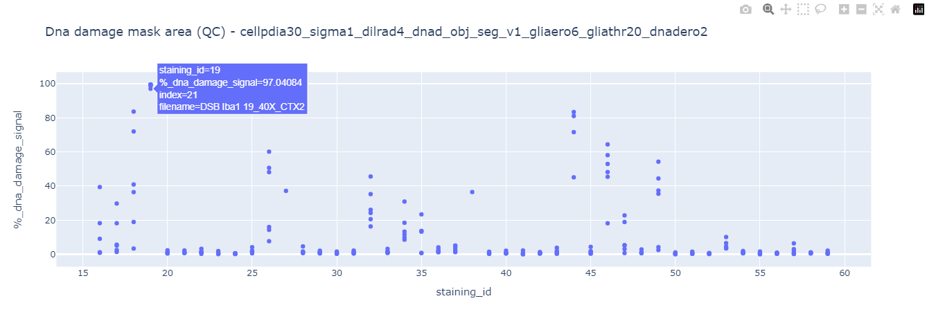
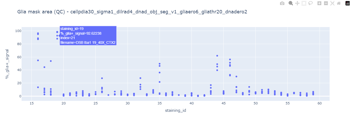
Afterwards it will display each technical replicate data point to explore the presence of outliers. This step is useful to detect errors in segmentation arising from poor quality data input (suboptimal stainings). Take a look at the DNA damage mask area and Glia mask area quality control plots. It is clear that a few of them show signs of aberrant segmentation, hovering the mouse over each data point will display the original filename and index.
Using the displayed index and applying the same analysis settings displayed in the graph titles in the 4_quality_checks.ipynb notebook we can observe how there is actually an issue with the input image (suboptimal stain with a lot of background). This notebook also outputs a Napari viewer for in detail exploration.
This 2data_exploration.ipynb notebook incorporates a QC (quality control) check based on these two analysis outputs (spot and cell marker mask areas). Any image where the value of those outputs is 3 times above the mean value of all samples will be flagged as a suboptimal stain and all datapoints associated with this particular staining_id will not pass QC. After performing this quality check a new qc.csv file will be generated containing all data points associated with their corresponding mouse_id data and stating the QC status staining_qc_passed = True / False. Based on this QC status the notebook will filter the datapoints that passed QC and display their corresponding graphs.
Both 3_qc_passed_image_display.ipynb and 3_qc_failed_image_display.ipynb notebooks take the same input as the 2_data_exploration.ipynb notebook.
- To analyze and pair microglia stainings you would type the following:
csv_path = "./results/results_cellpdia30_sigma1_dilrad4_dnad_obj_seg_v1_gliaero6_gliathr20_dnadero2.csv"
mouse_id_csv_path = "./mouse_ids_Iba1.csv"
- To analyze and pair astrocyte stainings you would type the following:
csv_path = "./results/results_cellpdia30_sigma1_dilrad4_dnad_obj_seg_v1_gliaero6_gliathr20_dnadero2.csv"
mouse_id_csv_path = "./mouse_ids_GFAP.csv"
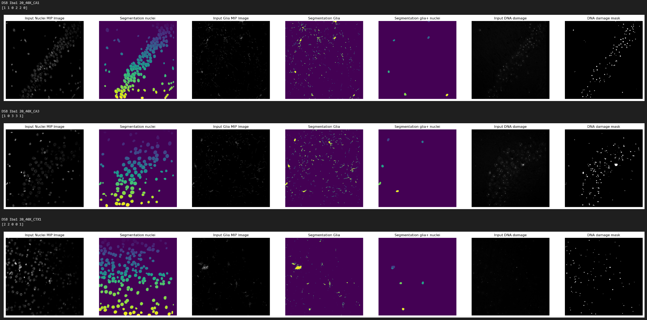
In this case the output will be different, both image display notebooks will extract the analysis settings from the results file and apply them to the images that passed or failed QC in a programmatic manner, then it will display them in-notebook for exploration as Matplotlib graphs. Preceding each analysis results you will find the associated filename and the number of spots detected inside each CM+ nucleus in a vector-like data structure [1 1 0 2 2 0].
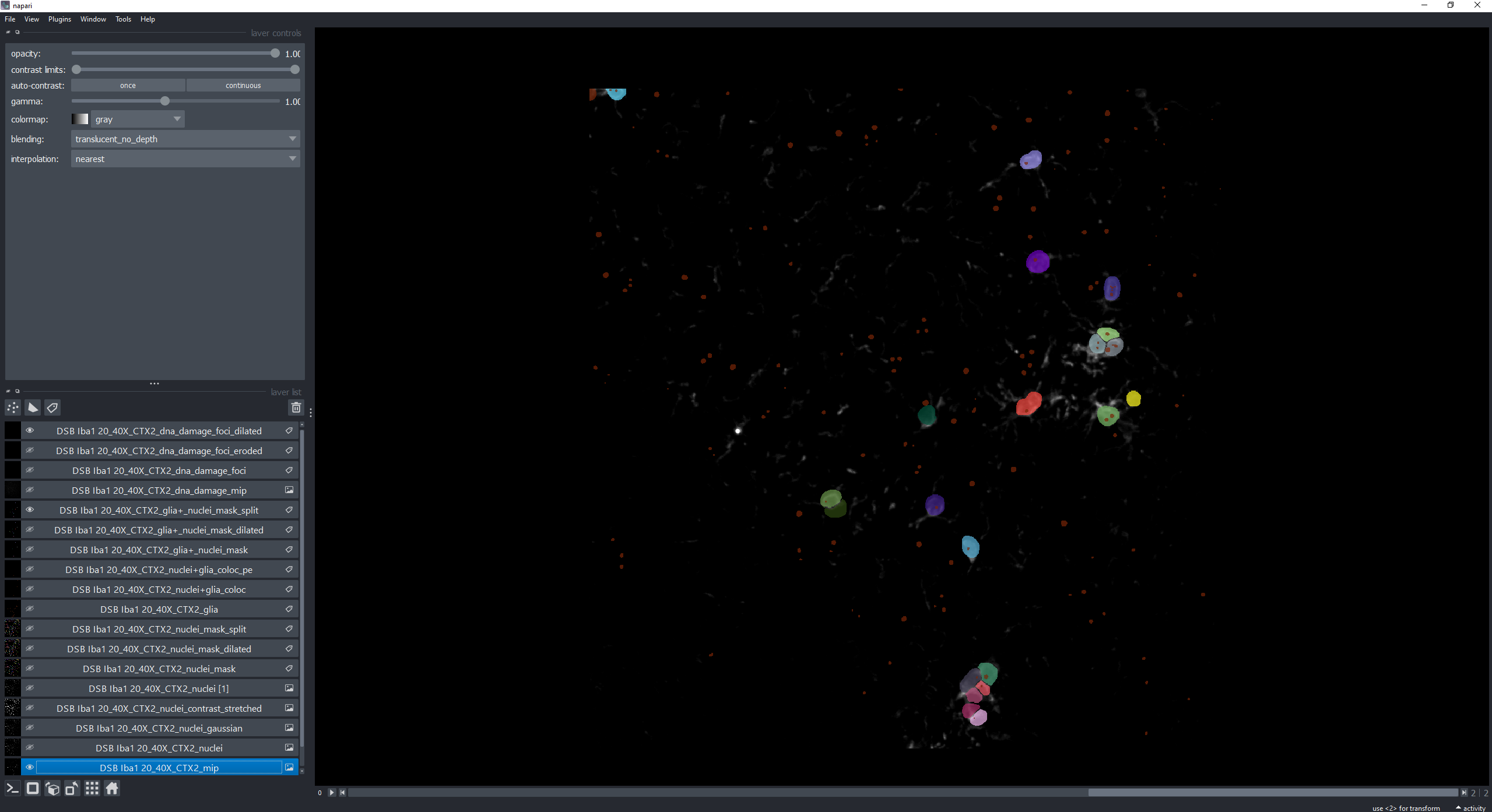
In order to play around with analysis parameters and display in detail resulting segmentations 4_quality_checks.ipynb allows to input the index of single images and to numerically tweak the analysis settings. On top of the Batch Image Data Exploration notebook outputs this notebook displays a Napari viewer that allows the visualization of every segmentation step in detail.
-
In order to run these Jupyter notebooks and .py scripts you will need to familiarize yourself with the use of Python virtual environments using Mamba. See instructions here.
-
Then you will need to create a virtual environment using the command below or from the .yml file in the envs folder (recommended, see step 3):
mamba create -n microglia python=3.9 devbio-napari cellpose pytorch torchvision plotly pyqt -c conda-forge -c pytorch -
To recreate the venv from the environment.yml file stored in the envs folder (recommended) navigate into the envs folder using
cdin your console and then execute:mamba env create -f environment.yml -
Activate it by typing in the console:
mamba activate microglia -
Then launch Jupyter lab to interact with the code by typing:
jupyter lab
