This is a project for Udacity self-driving car Nanodegree program. The aim of this project is to identify the lane in a dash camera video. The implementation of the project is in the file lane_detection.py, and the explanation of the pipeline is in this README and in lane_detection.ipynb. The final video output is here.
In this README, each step in the pipeline will be explained in details.
The pipeline for lane detection contains several steps:
- Correct image distortion.
- Image threshold to isolate lane lines in the image.
- Perspective transform to the "birds-eye view".
- Detect lane pixels.
- Fit to find the lane boundary.
- Determine the curvature of the lane and vehicle position with respect to center.
- Warp the detected lane boundaries back onto the original image and output visual display of the lane boundaries and position information.
In the following, each step in this pipeline will be described in detail.
The camera calibration step is aimed to remove the image distortion from the camera. In order to calibrate the camera, several check board images are taken using the same camera and are placed in the folder ./cameral_cal/. The distortion parameters are calculated using function
dist_mtx,dist_param = camera_cal_parameters(cal_images,image_size)
These parameters can then be used to correct the distortion in the images
image_undist = undistort(image,dist_mtx,dist_param))
The function camera_cal_parameters and undistort are based on the openCV function cv2.calibrateCamera and cv2.undistort. Here is the result of applying the undistortion to one of the calibration image
And here is the result of applying the correction to one of the test image
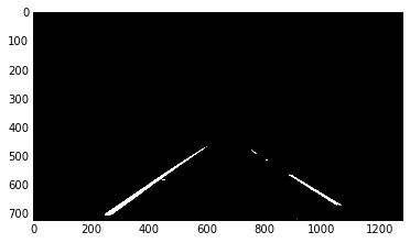
A binary image is generated using only color thresholds. The yellow lane lines and white lane lines are separated in different color spaces. The yellow lane line are separated in the C channel of LCH color space while the white lane lines are separated in the gray space. The reason to not use gradient filter is that color thresholds is much simpler and allows a cleaner separation and lower noises.
The thresholds can be applied to the image using the function
preprocess(image,mask_vertices,c_thresh,gray_thresh)
where mask_vertices is the vertices that defines the mask region, c_thresh and gray_thresh are the thresholds in C channel and gray channel, respectively. This is the result of applying the function to the same test image above
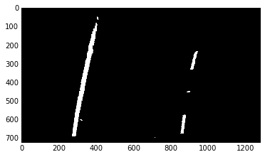
In order to fit the lane lines, the image is transformed into the "birds-eye" perspective. The function that performs this transformation is
perspective_transform(image_binary,src,dst)
where src defines the source points in the original image and dst defines the destination points in the "bird-eye" image. The source and destination points used in the code are
| Source | Destination |
|---|---|
| 258, 679 | 258, 679 |
| 446, 549 | 258, 549 |
| 837, 549 | 837, 549 |
| 1045, 679 | 837, 679 |
After the perspective transform, the two lane lines should be approximately in parallel, and that's the case for our transform
The procedures to detect lane pixels are:
- Select the bottom half of the image, and obtain a histogram for the intensity as a function of the X value.
- Smooth this histogram using a Gaussian filter, and identify the two peaks using the
find_peaks_cwtfromscipy.signal. These two peaks will be used as the initial position of the sliding windows for the left and right lane lines. - Apply a sliding window with certain width and height to the lef and right lane lines. Calculate the histogram in those windows, and find the centers of left and right lane lines using the
center_of_massfunction inscipy.ndimage.measurements. These new centers will be used as the position for the next sliding windows. - Repeat the above step and moving the sliding window up by the amount of the window height, until it reaches to the height of the image.
These procedures can be applied using the function
select_lane_lines(warped_lane,sliding_window)
where sliding_window is the dimension for the sliding window, and is set to [80,120] in the code. Here is the result of applying the function to the same test image
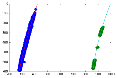
After separating the left and right lane line pixels, the lane boundary can be found by fitting to a second order polynomial. This fitting process can be done using the function
fit_lane_line(lr_binary_images)
where lr_binary_images is the binary image for the left and right lane lines. This function is based on the numpy function np.polyfit. This shows the fitted lane lines
The radius of curvature is determined by
, and for our function
the radius becomes
The position with respect to center can be calculated by evaluating the fitted function at the bottom of the image and compares that to the center of the image. The curvature and the position can be calculated using the function
cal_curvature(lr_binary_images)
Once we detect the lane in the "bird-eye" view, we can wrap that back to the original image perspective. This can be done using the function
draw_lane(image,left_right_fits,src,dst)
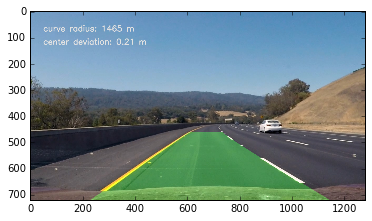
where image is the original image, left_right_fits are the polynomial fits for the left and right lane lines, src and dst are the transformation points. The information of the lane curvature radius and vehicle position can be printed onto the image using
print_info(image,radius,deviation)
The result of applying these two functions is
This pipeline for a single image can be applied to the video the same way.
Here's a link to the video result
The most critical part in this project is to generate a binary image that detects the lane lines. This is non-trivial for complicated lighting situations. In the current implementation, detecting lane lines are achieved by using only the color thresholds. By using only the color thresholds, the resulted image are much more clean and easier to process than the gradient filtered one. The color thresholds are based on the assumption that the lane line is either yellow or white, and it appears to work very well for the video provided. However, color thresholds alone are not enough for the situation where the lane lines colors are changed dramatically under complicated lighting situations. For future improvements, combining color and gradient filters may lead better results.


