Ballgown is a software package designed to facilitate flexible differential expression analysis of RNA-Seq data. It also provides functions to organize, visualize, and analyze the expression measurements for your transcriptome assembly.
Before using the Ballgown R package, a few preprocessing steps are necessary:
- RNA-Seq reads should be aligned to a reference genome.
- A transcriptome should be assembled, or a reference transcriptome should be downloaded.
- Expression for the features (transcript, exon, and intron junctions) in the transcriptome should be estimated in a Ballgown readable format.
Two sample pipelines for preprocessing are as follows:
- Pipeline 1: TopHat2 (1) + Stringtie (2,3)
- TopHat2 [Trapnell et al. (2009)] is built on the ultrafast short read mapping program Bowtie and aligns RNA-Seq reads to a genome while identifying exonic splice junctions. Sample command:
tophat2 -G reference.gff -o outputDirectory -p 6 referenceIndex reads - Stringtie [M. Pertea et al. (2015)] is a highly efficient assembler for RNA-Seq alignments using a novel network flow algorithm. It simultaneously assembles and quantifies expression levels for the features of the transcriptome in a Ballgown readable format (by using the option -B). One command to Stringtie satisfies steps 2 and 3 above. Sample command:
stringtie -B -G reference.gff -p 6 accepted_hits.bam -o stringtie.gff - Pipeline 2: TopHat2 (1) + Cufflinks (2) + Tablemaker (3)
- Tophat2 produces alignments as noted above.
- Cufflinks [Trapnell et al. (2010)] also assembles transcriptomes from RNA-Seq data and quantifies their expression. Sample command:
cufflinks -g reference.gff -o outputDirectory accepted_hits.bam - Tablemaker calls Cufflinks to estimate feature expressions in a Ballgown readable format. Tablemaker access and instructions can be found here.
Start R and run:
if (!requireNamespace("BiocManager", quietly=TaRUE))
    install.packages("BiocManager")
BiocManager::install("ballgown")The files that Stringtie and Tablemaker produce for Ballgown to load is as follows:
e_data.ctab: exon-level expression measurements. One row per exon. Columns aree_id(numeric exon id),chr,strand,start,end(genomic location of the exon), and the following expression measurements for each sample:rcount: reads overlapping the exonucount: uniquely mapped reads overlapping the exonmrcount: multi-map-corrected number of reads overlapping the exoncovaverage per-base read coveragecov_sd: standard deviation of per-base read coveragemcov: multi-map-corrected average per-base read coveragemcov_sd: standard deviation of multi-map-corrected per-base coverage
i_data.ctab: intron- (i.e., junction-) level expression measurements. One row per intron. Columns arei_id(numeric intron id),chr,strand,start,end(genomic location of the intron), and the following expression measurements for each sample:rcount: number of reads supporting the intronucount: number of uniquely mapped reads supporting the intronmrcount: multi-map-corrected number of reads supporting the intron
t_data.ctab: transcript-level expression measurements. One row per transcript. Columns are:t_id: numeric transcript idchr,strand,start,end: genomic location of the transcriptt_name: Cufflinks-generated transcript idnum_exons: number of exons comprising the transcriptlength: transcript length, including both exons and intronsgene_id: gene the transcript belongs togene_name: HUGO gene name for the transcript, if knowncov: per-base coverage for the transcript (available for each sample)FPKM: Cufflinks-estimated FPKM for the transcript (available for each sample)
e2t.ctab: table with two columns,e_idandt_id, denoting which exons belong to which transcripts. These ids match the ids in thee_dataandt_datatables.i2t.ctab: table with two columns,i_idandt_id, denoting which introns belong to which transcripts. These ids match the ids in thei_dataandt_datatables.
The default directory structure produced by Stringtie and Tablemaker should mirror the extdata folder in the Ballgown pacakge:
extdata/
    sample01/
        e2t.ctab
        e_data.ctab
        i2t.ctab
        i_data.ctab
        t_data.ctab
    sample02/
        e2t.ctab
        e_data.ctab
        i2t.ctab
        i_data.ctab
        t_data.ctab
    ...
    sample20/
        e2t.ctab
        e_data.ctab
        i2t.ctab
        i_data.ctab
        t_data.ctab
Data is loaded using the ballgown function.
If your data is stored in directories matching the above structure (one root folder, subfolders named by sample, and .ctab files in the subfolders), you can use the dataDir and samplePattern arguments to load the data. samplePattern takes a regular expressions specifying the subfolders that should be included in the ballgown object:
library(ballgown)
data_directory = system.file('extdata', package='ballgown') # automatically finds ballgown's installation directory
# examine data_directory:
data_directory
## [1] "/Library/Frameworks/R.framework/Versions/3.1/Resources/library/ballgown/extdata"
# make the ballgown object:
bg = ballgown(dataDir=data_directory, samplePattern='sample', meas='all')
bg
## ballgown instance with 100 transcripts and 20 samples
If your data is stored in a directory structure other than the one specified above, you can use the samples argument in the ballgown function: samples should be a vector (1-d array) with one entry per sample, where the entry gives the path to the folder containing that sample's .ctab files.
The result from either of these approaches is an object of class ballgown (named bg in these examples).
In the rest of this document, we use bg to refer to the first example, where samples are named sample01 through sample20.
A note for large experiments (with many samples or with large genomes): loading the data might require a lot of time and memory. In these cases, it's often useful to do the data loading in non-interactive mode. More specifically, you could create a script called load.R that contains these lines:
library(ballgown)
data_directory = system.file('extdata', package='ballgown')
bg = ballgown(dataDir=data_directory, samplePattern='sample', meas='all')
save(bg, file='bg.rda')
You could then run this script non-interactively using R CMD BATCH: from the command line, run:
R CMD BATCH load.R
This may take some time, but when it finishes, the file bg.rda will be saved in the current directory, and you can read it back into R using the load() function. Rda files are usually only a few Gb on disk, even for large experiments. It is also possible to load only a subset of all the expression measurements by changing the meas argument to the ballgown function. For example, to only load transcript-level FPKMs, set meas = 'FPKM' and to load average coverage values and read counts, set meas=c('cov', 'rcount').
See ?ballgown for detailed information on creating Ballgown objects.
A ballgown object has six slots: structure, expr, indexes, dirs, mergedDate, and meas.
The structure slot depends heavily on the GenomicRanges Bioconductor package (Lawrence et al. (2013)). The slot specifies the structure, i.e., genomic locations and relationships between exons, introns, and transcripts, of the transcriptome assembly. It is convenient to represent exons and introns as intervals and to represent transcripts as a set of intervals (exons), so assembled exons and introns are available as GRanges objects, and the assembled transcripts are available as a GRangesList object. This means that useful range operations, such as findOverlaps and reduce, are readily available for assembled features.
Exon, intron, and transcript structures are easily extracted from the main ballgown object:
structure(bg)$exon## GRanges object with 633 ranges and 2 metadata columns:
## seqnames ranges strand | id transcripts
## <Rle> <IRanges> <Rle> | <integer> <character>
## [1] 18 [24412069, 24412331] * | 12 10
## [2] 22 [17308271, 17308950] + | 55 25
## [3] 22 [17309432, 17310226] + | 56 25
## [4] 22 [18121428, 18121652] + | 88 35
## [5] 22 [18138428, 18138598] + | 89 35
## ... ... ... ... ... ... ...
## [629] 22 [51221929, 51222113] - | 3777 1294
## [630] 22 [51221319, 51221473] - | 3782 1297
## [631] 22 [51221929, 51222162] - | 3783 1297
## [632] 22 [51221929, 51222168] - | 3784 1301
## [633] 6 [31248149, 31248334] * | 3794 1312
## -------
## seqinfo: 3 sequences from an unspecified genome; no seqlengths
structure(bg)$intron## GRanges object with 536 ranges and 2 metadata columns:
## seqnames ranges strand | id
## <Rle> <IRanges> <Rle> | <integer>
## [1] 22 [17308951, 17309431] + | 33
## [2] 22 [18121653, 18138427] + | 57
## [3] 22 [18138599, 18185008] + | 58
## [4] 22 [18185153, 18209442] + | 59
## [5] 22 [18385514, 18387397] - | 72
## ... ... ... ... ... ...
## [532] 22 [51216410, 51220615] - | 2750
## [533] 22 [51220776, 51221928] - | 2756
## [534] 22 [51220780, 51221318] - | 2757
## [535] 22 [51221474, 51221928] - | 2758
## [536] 22 [51220780, 51221928] - | 2759
## transcripts
## <character>
## [1] 25
## [2] 35
## [3] 35
## [4] 35
## [5] 41
## ... ...
## [532] c(1294, 1297, 1301)
## [533] 1294
## [534] 1297
## [535] 1297
## [536] 1301
## -------
## seqinfo: 1 sequence from an unspecified genome; no seqlengths
structure(bg)$trans## GRangesList object of length 100:
## $10
## GRanges object with 1 range and 2 metadata columns:
## seqnames ranges strand | id transcripts
## <Rle> <IRanges> <Rle> | <integer> <character>
## [1] 18 [24412069, 24412331] * | 12 10
##
## $25
## GRanges object with 2 ranges and 2 metadata columns:
## seqnames ranges strand | id transcripts
## [1] 22 [17308271, 17308950] + | 55 25
## [2] 22 [17309432, 17310226] + | 56 25
##
## $35
## GRanges object with 4 ranges and 2 metadata columns:
## seqnames ranges strand | id transcripts
## [1] 22 [18121428, 18121652] + | 88 35
## [2] 22 [18138428, 18138598] + | 89 35
## [3] 22 [18185009, 18185152] + | 90 35
## [4] 22 [18209443, 18212080] + | 91 35
##
## ...
## <97 more elements>
## -------
## seqinfo: 3 sequences from an unspecified genome; no seqlengths
The expr slot is a list that contains tables of expression data for the genomic features. These tables are very similar to the *_data.ctab Tablemaker output files. Ballgown implements the following syntax to access components of the expr slot:
*expr(ballgown_object_name, <EXPRESSION_MEASUREMENT>)where * is either e for exon, i for intron, t for transcript, or g for gene, and is an expression-measurement column name from the appropriate .ctab file. Gene-level measurements are calculated by aggregating the transcript-level measurements for that gene. All of the following are valid ways to extract expression data from the bg ballgown object:
transcript_fpkm = texpr(bg, 'FPKM')
transcript_cov = texpr(bg, 'cov')
whole_tx_table = texpr(bg, 'all')
exon_mcov = eexpr(bg, 'mcov')
junction_rcount = iexpr(bg)
whole_intron_table = iexpr(bg, 'all')
gene_expression = gexpr(bg)
Calculating the gene-level expression measurements can be slow for large experiments.
The *expr functions return matrices unless meas = 'all', in which case some additional feature metadata is returned and the result is a data.frame.
The indexes slot of a ballgown object connects the pieces of the assembly and provides other experimental information. indexes(bg) is a list with several components that can be extracted with the $ operator.
Perhaps most importantly, there is a component called pData that should hold a data frame of phenotype information for the samples in the experiment. This must be created manually. It is very important that the rows of pData are in the correct order. Each row corresponds to a sample, and the rows of pData should be ordered the same as the tables in the expr slot. You can check that order by running sampleNames(bg). The pData component can be added during construction (you can pass a data frame to the ballgown function), or you can add it later:
pData(bg) = data.frame(id=sampleNames(bg), group=rep(c(1,0), each=10))The other components of indexes are the e2t and i2t tables described in the Tablemaker section, as well as a t2g table denoting which transcripts belong to which genes. There is also a bamfiles component, designed to hold paths to the read alignment files for each sample. The bamfiles component isn't currently used by any ballgown functions, but it could come in handy for users of RSamtools or similar packages. Here are some examples of how to extract indexes components from ballgown objects:
exon_transcript_table = indexes(bg)$e2t
transcript_gene_table = indexes(bg)$t2g
head(transcript_gene_table)
## t_id g_id
## 1 10 XLOC_000010
## 2 25 XLOC_000014
## 3 35 XLOC_000017
## 4 41 XLOC_000246
## 5 45 XLOC_000019
## 6 67 XLOC_000255
phenotype_table = pData(bg)The dirs slot gives full filepaths to Tablemaker output:
head(bg@dirs)## sample01
## "/Library/Frameworks/R.framework/Versions/3.1/Resources/library/ballgown/extdata/sample01"
## sample02
## "/Library/Frameworks/R.framework/Versions/3.1/Resources/library/ballgown/extdata/sample02"
## sample03
## "/Library/Frameworks/R.framework/Versions/3.1/Resources/library/ballgown/extdata/sample03"
## sample04
## "/Library/Frameworks/R.framework/Versions/3.1/Resources/library/ballgown/extdata/sample04"
## sample05
## "/Library/Frameworks/R.framework/Versions/3.1/Resources/library/ballgown/extdata/sample05"
## sample06
## "/Library/Frameworks/R.framework/Versions/3.1/Resources/library/ballgown/extdata/sample06"
The mergedDate slot indicates when the ballgown object was created:
bg@mergedDate## [1] "Sun Feb 22 23:51:45 2015"
And the meas slot gives the expression measurements present in the object:
bg@meas## [1] "all"
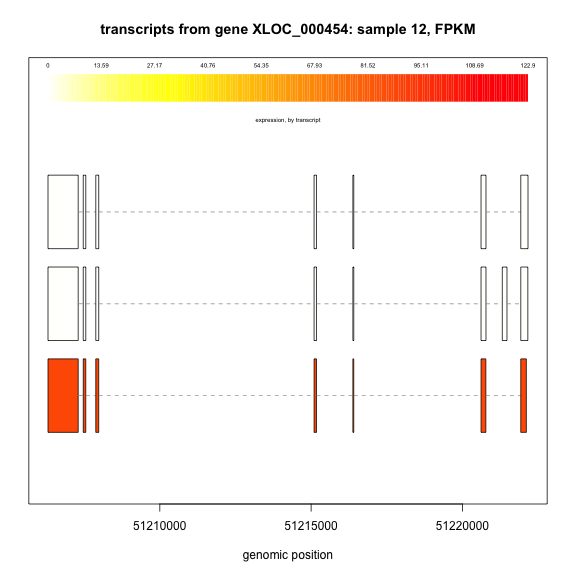
Visualization of the assembled transcripts is done with the plotTranscripts function. Transcripts or exons can be colored by expression level. This plot colors transcripts by expression level:
plotTranscripts(gene='XLOC_000454', gown=bg, samples='sample12',
    meas='FPKM', colorby='transcript',
    main='transcripts from gene XLOC_000454: sample 12, FPKM')
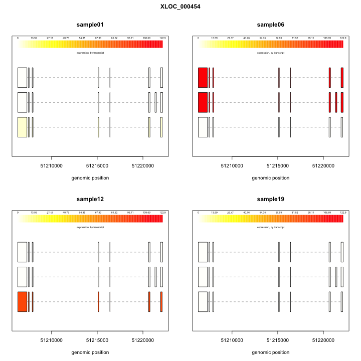
It is also possible to plot several samples at once:
plotTranscripts('XLOC_000454', bg,
    samples=c('sample01', 'sample06', 'sample12', 'sample19'),
    meas='FPKM', colorby='transcript')
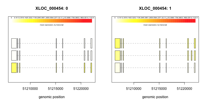
You can also make side-by-side plots comparing mean abundances between groups (here, 0 and 1):
plotMeans('XLOC_000454', bg, groupvar='group', meas='FPKM', colorby='transcript')Ballgown provides a wide selection of simple, fast statistical methods for testing whether transcripts are differentially expressed between experimental conditions or across a continuous covariate (such as time).
The default statistical test in ballgown is a parametric F-test comparing nested linear models; details are available in the Ballgown manuscript (Frazee et al. (2014)). These models are conceptually simialar to the models used by Smyth (2005) in the limma package. In limma, more sophisticated empirical Bayes shrinkage methods are used, and generally a single linear model is fit per feature instead of doing a nested model comparison, but the flavor is similar (and in fact, limma can easily be run on any of the data matrices in a ballgown object).
Ballgown's statistical models are implemented with the stattest function. Two models are fit to each feature, using expression as the outcome: one including the covariate of interest (e.g., case/control status or time) and one not including that covariate. An F statistic and p-value are calculated using the fits of the two models. A significant p-value means the model including the covariate of interest fits significantly better than the model without that covariate, indicating differential expression. We adjust for multiple testing by reporting q-values (Storey & Tibshirani (2003)) for each transcript in addition to p-values: reporting features with, say, q < 0.05 means the false discovery rate should be controlled at about 5%.
stattest automatically handles two-group (e.g. case/control) comparisons, multi-group comparisons (e.g. comparison of several tissue types), and "timecourse" comparisons (with the scare quotes meaning that these comparisons are also applicable to continuous covariates that aren't time). For two- and multi-group comparisons, a significant result indicates that the feature is differentially expressed in at least one of the groups. For timecourse comparisons, significant results mean the feature has an expression profile that varies significantly over time (i.e., values of the continuous covariate) as opposed to being flat over time.
The example dataset bg contains two group labels, 0 and 1. We can test each transcript for differential expression with stattest:
stat_results = stattest(bg, feature='transcript', meas='FPKM', covariate='group')
head(stat_results)
## feature id pval qval
## 1 transcript 10 0.01381576 0.10521233
## 2 transcript 25 0.26773622 0.79114975
## 3 transcript 35 0.01085070 0.08951825
## 4 transcript 41 0.47108019 0.90253747
## 5 transcript 45 0.08402948 0.48934813
## 6 transcript 67 0.27317385 0.79114975
The result is a data frame containing the feature tested, feature ids, and corresponding p- and q-values. See ?stattest for further usage details.
For timecourse experiments, a smooth curve is fit to time (or the continuous covariate) using natural splines. The default degrees of freedom used for the spline model is 4, but this can be adjusted with the df option. The model for expression including these spline terms is compared to a model without any spline terms for the F-test. The results indicate which features' expression levels change significantly over time. For our example, we can define a "time" covariate and then demonstrate a typical call to stattest for a timecourse experiment:
pData(bg) = data.frame(pData(bg), time=rep(1:10, 2)) #dummy time covariate
timecourse_results = stattest(bg, feature='transcript', meas='FPKM', covariate='time', timecourse=TRUE)
The timecourse option assumes that "time" in your study is truly continuous, i.e., that it takes several values along a time scale. If you have very few timepoints (e.g., fewer than 5), we recommend treating time as a categorical variable, since having very few values does not give much granularity for fitting a smooth curve using splines. You can do this by setting covariate equal to 'time' (or whatever your time variable is named) and simply leaving timecourse as FALSE, its default. If you don't have more timepoints than degrees of freedom in the spline model, a warning will be printed and time will be coerced to categorical.
You can adjust for any or all variables in pData when testing for differential expression. Ballgown automatically adjusts for library size using the sum of all logged nonzero expression measurements below the 75th percentile of those measurements, for each sample. If you would like to adjust for other variables, just provide those confounders as the adjustvars argument to stattest:
group_adj_timecourse_results = stattest(bg, feature='transcript', meas='FPKM', covariate='time',
timecourse=TRUE, adjustvars='group')It is also possible to explicitly provide the design matrices for the models to be compared. For example, suppose we had sex and age information available, in addition to group and time, and we wanted to compare a model including all information (sex, age, group, time) to a model including only group and time. Code to do this with ballgown is:
# create example data:
set.seed(43)
sex = sample(c('M','F'), size=nrow(pData(bg)), replace=TRUE)
age = sample(21:52, size=nrow(pData(bg)), replace=TRUE)

# create design matrices:
mod = model.matrix(~ sex + age + pData(bg)$group + pData(bg)$time)
mod0 = model.matrix(~ pData(bg)$group + pData(bg)$time)

# run differential expression tests:
adjusted_results = stattest(bg, feature='transcript', meas='FPKM', mod0=mod0, mod=mod)
head(adjusted_results)
## feature id pval qval
## 1 transcript 10 0.8242859 0.9755925
## 2 transcript 25 0.1985488 0.9725569
## 3 transcript 35 0.8114314 0.9755925
## 4 transcript 41 0.7647284 0.9755925
## 5 transcript 45 0.6497589 0.9755925
## 6 transcript 67 0.9775119 0.9874866
Ballgown's statistical methods for differential expression testing are straightforward and accurate (Frazee et al. (2014)), but users may wish to use one of the many existing packages for differential expression. Ballgown's data structures make it easy to use table-based packages like limma (Smyth (2005)), limma Voom (Law et al. (2014)), DESeq (Anders & Huber (2010)), DEXSeq (Anders et al. (2012)), or EdgeR (Robinson et al. (2010)) for differential expression analysis. A feature-by-sample expression table can be easily created with a *expr function and used directly as input to these or other differential expression packages.
Sometimes several very similar transcripts are assembled for the same gene, which might cause expression estimates for those transcripts to be unreliable: statistically, it can very difficult or impossible to tell which of two very similar transcript a read came from. This means differential expression results might also be unreliable.
As a preliminary attempt at addressing this issue, Ballgown provides some simple transcript clustering functions. The idea is that similar assembled transcripts can be grouped together in clusters, and differential expression analysis could be performed on the cluster, whose expression measurement aggregates the expression estimates of the transcripts that compose it.
These functions measure the distance between transcripts using Jaccard distance, where each transcript's "set" is the nucleotides included in its exons. Transcripts can be clustered using either k-means clustering or hierarchical clustering.
clusterTranscripts(gene='XLOC_000454', gown=bg, k=2, method='kmeans')## $clusters
## cluster t_id
## 1 2 1294
## 2 1 1297
## 3 2 1301
##
## $pctvar
## [1] 0.9117737
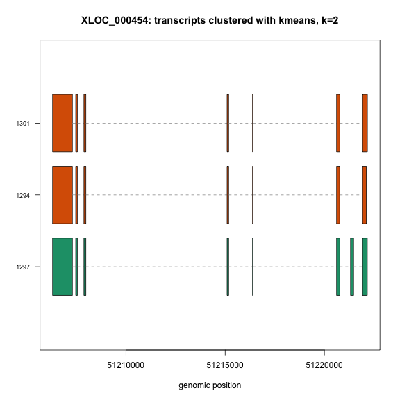
You can also visualize the transcript clusters:
plotLatentTranscripts(gene='XLOC_000454', gown=bg, k=2, method='kmeans', returncluster=FALSE)And you can calculate aggregate cluster expression measurements for some gene using collapseTranscripts. The tab result of collapseTranscripts can be passed to stattest as the gowntable argument, for differential expression analysis of the clusters:
agg = collapseTranscripts(gene='XLOC_000454', gown=bg, k=2, method='kmeans')
stattest(gowntable=agg$tab, pData=pData(bg), feature='transcript_cluster',
    covariate='group', libadjust=FALSE)
## feature id pval qval
## 1 transcript_cluster 1 0.3332238 0.6664477
## 2 transcript_cluster 2 0.6882119 0.6882119
This example clustered only three transcripts, but we imagine clustering could be useful when many more than three transcripts have been assembled for a single gene.
- Simon Anders, Wolfgang Huber (2010). Differential Expression Analysis For Sequence Count Data. Genome Biology 11 R106-NA 10.1186/gb-2010-11-10-r106
- Simon Anders, Alejandro Reyes, Wolfgang Huber (2012). Detecting Differential Usage of Exons From RNA-Seq Data. Genome Research 22 2008-2017 10.1101/gr.133744.111
- Alyssa C. Frazee, Geo Pertea, Andrew E. Jaffe, Ben Langmead, Steven L. Salzberg, Jeffrey T. Leek (2014). Flexible isoform-level differential expression analysis with Ballgown. bioRxiv http://biorxiv.org/content/early/2014/03/30/003665
- Charity W Law, Yunshun Chen, Wei Shi, Gordon K Smyth, (2014) Voom: Precision Weights Unlock Linear Model Analysis Tools For RNA-Seq Read Counts. Genome Biology 15 R29-NA 10.1186/gb-2014-15-2-r29
- Michael Lawrence, Wolfgang Huber, Herve Pages, Patrick Aboyoun, Marc Carlson, Robert Gentleman, Martin T. Morgan, Vincent J. Carey, Andreas Prlic (2013). Software For Computing And Annotating Genomic Ranges. Plos Computational Biology 9 e1003118-NA 10.1371/journal.pcbi.1003118
- Mihaela Pertea, Geo M Pertea, Corina M Antonescu, Tsung-Cheng Chang, Joshua T Mendell, Steven L Salzberg (2015). StringTie enables improved reconstruction of a transcriptome from RNA-seq reads. Nature Biotechnology http://www.nature.com/nbt/journal/v33/n3/full/nbt.3122.html
- Mark D. Robinson, Davis J. McCarthy and Gordon K. Smyth (2009) "edgeR: a Bioconductor package for differential expression analysis of digital gene expression data". Bioinformatics 26.1 pp. 139-140. 10.1093/bioinformatics/btp616
- Gordon Smyth, (2005) Limma: linear models for microarray data. 397-420
- John D. Storey, Robert Tibshirani (2003). Statistical Significance For Genomewide Studies. Proceedings of The National Academy of Sciences 100 9440-9445 10.1073/pnas.1530509100
- Cole Trapnell, Lior Pachter, Steven Salzberg (2009) TopHatL discovering splice junctions with RNA-Seq. Bioinformatics. [http://bioinformatics.oxfordjournals.org/content/25/9/1105.abstract] (http://bioinformatics.oxfordjournals.org/content/25/9/1105.abstract)
- Cole Trapnell, Brian A Williams, Geo Pertea, Ali Mortazavi, Gordon Kwan, Marijke J van Baren, Steven L Salzberg, Barbara J Wold, Lior Pachter (2010) Transcript Assembly And Quantification by Rna-Seq Reveals Unannotated Transcripts And Isoform Switching During Cell Differentiation. Nature Biotechnology 28 511-515 10.1038/nbt.1621
sessionInfo()## R version 3.1.1 (2014-07-10)
## Platform: x86_64-apple-darwin13.1.0 (64-bit)
##
## locale:
## [1] en_US.UTF-8/en_US.UTF-8/en_US.UTF-8/C/en_US.UTF-8/en_US.UTF-8
##
## attached base packages:
## [1] stats graphics grDevices utils datasets methods base
##
## other attached packages:
## [1] ballgown_1.0.1 knitr_1.8.2 colorout_1.0-3 devtools_1.6.1
##
## loaded via a namespace (and not attached):
## [1] annotate_1.44.0 AnnotationDbi_1.28.1
## [3] base64enc_0.1-2 BatchJobs_1.5
## [5] BBmisc_1.8 Biobase_2.26.0
## [7] BiocGenerics_0.12.1 BiocParallel_1.0.0
## [9] Biostrings_2.34.0 bitops_1.0-6
## [11] brew_1.0-6 checkmate_1.5.0
## [13] codetools_0.2-9 DBI_0.3.1
## [15] digest_0.6.4 evaluate_0.5.5
## [17] fail_1.2 foreach_1.4.2
## [19] formatR_1.0 genefilter_1.48.1
## [21] GenomeInfoDb_1.2.3 GenomicAlignments_1.2.1
## [23] GenomicRanges_1.18.3 grid_3.1.1
## [25] IRanges_2.0.0 iterators_1.0.7
## [27] lattice_0.20-29 limma_3.22.1
## [29] Matrix_1.1-4 mgcv_1.8-4
## [31] nlme_3.1-118 parallel_3.1.1
## [33] RColorBrewer_1.1-2 RCurl_1.95-4.5
## [35] Rsamtools_1.18.2 RSQLite_1.0.0
## [37] rtracklayer_1.26.2 S4Vectors_0.4.0
## [39] sendmailR_1.2-1 splines_3.1.1
## [41] stats4_3.1.1 stringr_0.6.2
## [43] survival_2.37-7 sva_3.12.0
## [45] tools_3.1.1 XML_3.98-1.1
## [47] xtable_1.7-4 XVector_0.6.0
## [49] zlibbioc_1.12.0


