As part of our CSE567: Principles Of Digital Systems Design class at University of Washington, we seek to improve a part of the BlackParrot Open-Source RISC-V processor in terms of PPA (Power, Performance, Area) and/or simplicity. We decided to tackle the problem of improving the branch predictor, since a better predictor can easily improve the overall performance by reducing the number of misspredictions/revertions.
The current implementation is a fixed-width (=2) saturating counter one-level bimodal branch predictor. In order to explore the whole design space, we generalized the existing implementation by imposing an adjustable saturating counter bit-width parameter on the one hand, and we implemented different branch predictors such as always-taken, gselect, gshare, two-level local and tournament on the other hand. The major contribution is not only the RTL implementation of these predictors, but also a comprehensive study and comparison in terms of prediction performance and PPA between the designs. Furthermore, we seek to show that modern and good coding practices from high-level languages such as continuous-integration can be applied on hardware design too.
To gain the ability of comparison between the different implementations, we first started with the existing test programs of black parrot, which reports the number of cycles for each test program execution (verilator simulation). This approach comes with a couple of downsides.
(1) Firstly, we are reporting cycles instead of accuracy (#correct predictions/#total branches). This is problematic in multiple ways, e.g. what if the program does not contain any branches/only very few? what if the branches are only of a certain type?
(2) Secondly, some of the test programs finish execution in only a few thousand cycles, while only a fraction of these cycles are spent on branch instructions. This drastically reduces the statistical relevance of our findings from these tests.
(3) Last but not least, since malfunctioning branch predictors only decrease the performance, but not the correct code execution we have no notion of testing the correctness of our implementation. Recall: "Hardware is about 10x as hard to debug as software.", Part of Taylor's VLSI Axiom #5. In the case of a branch predictor, with a large internal state, it is even almost impossible to write good tests by hand.
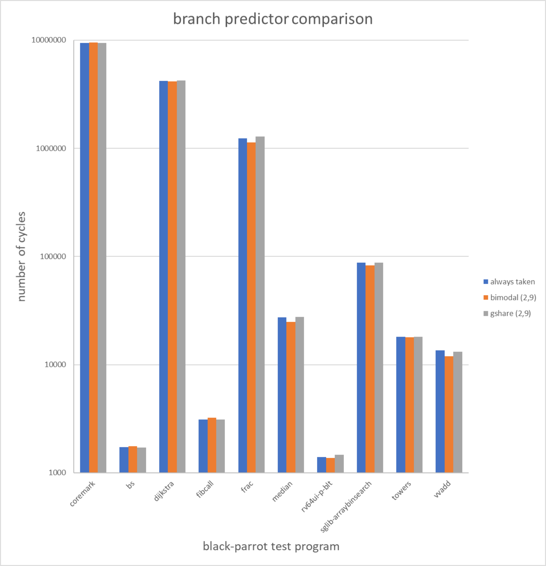
This reasoning above can be underlined well with one of our early cycle performance analysis. Even for larger tests such
as the coremark benchmark, we even get slightly better performance (lower cycle count is better) with the primitive
'always taken' implementation compared to the current 'bimodal' branch predictor.
In order to overcome these limitations, we developed our own performance evaluation and testing system.
After receiving a hint from Professor Taylor, we started investigating the use of branch traces from the most recent
Championship Branch Prediction CBP-5. Since these files come in a complex encoding scheme, we
used their branch predictor test backbone and built a conversion utility that translates these files to a simple "branch_address branch_taken newline" format. The implementation details can be found in bt9_reader. For our evaluation and simulation, we used four of the training files from different categories (short_mobile_1, long_mobile_1, short_server_1, long_server_1), each consisting of several millions of branches. The converted files can be found in traces.
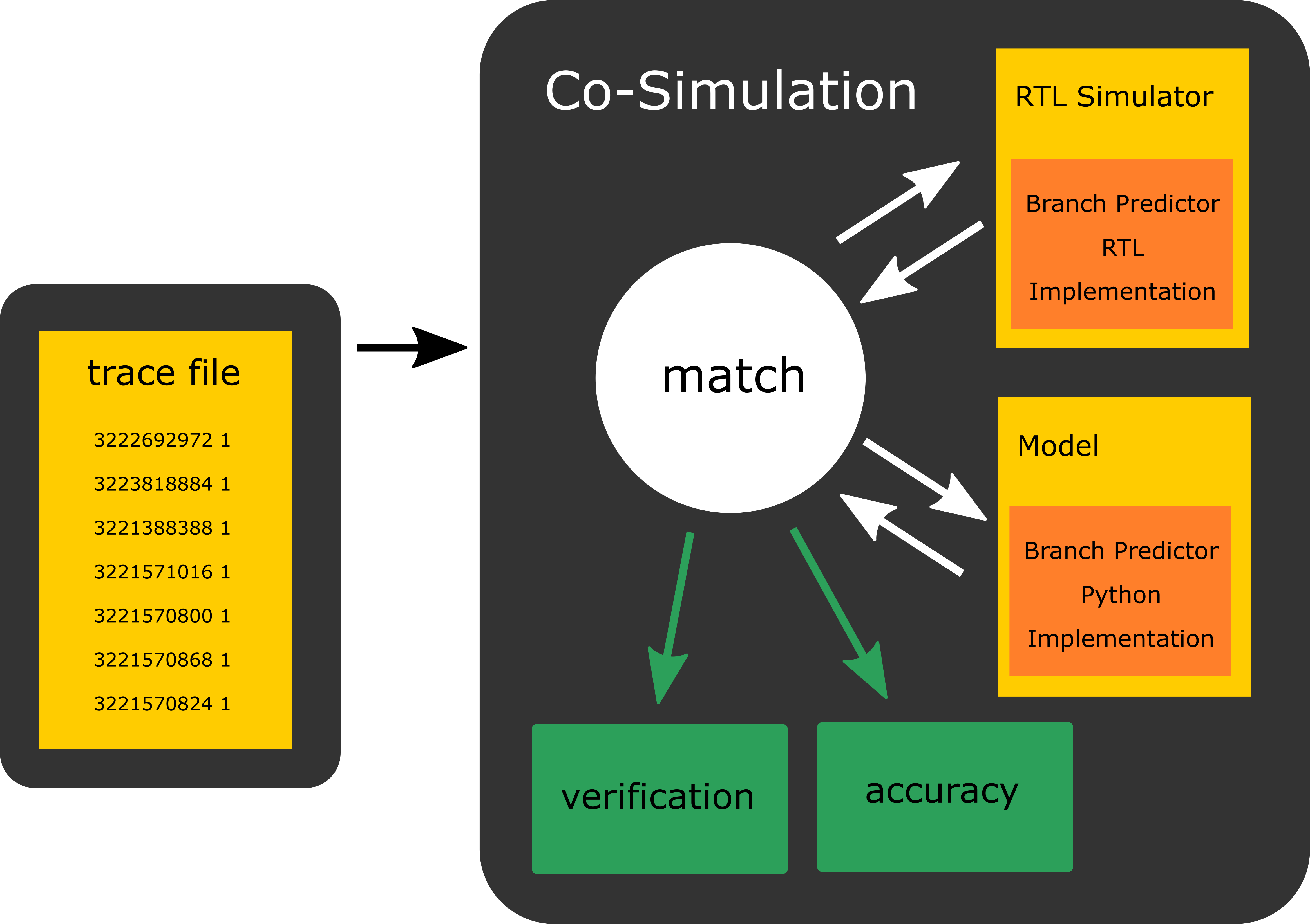
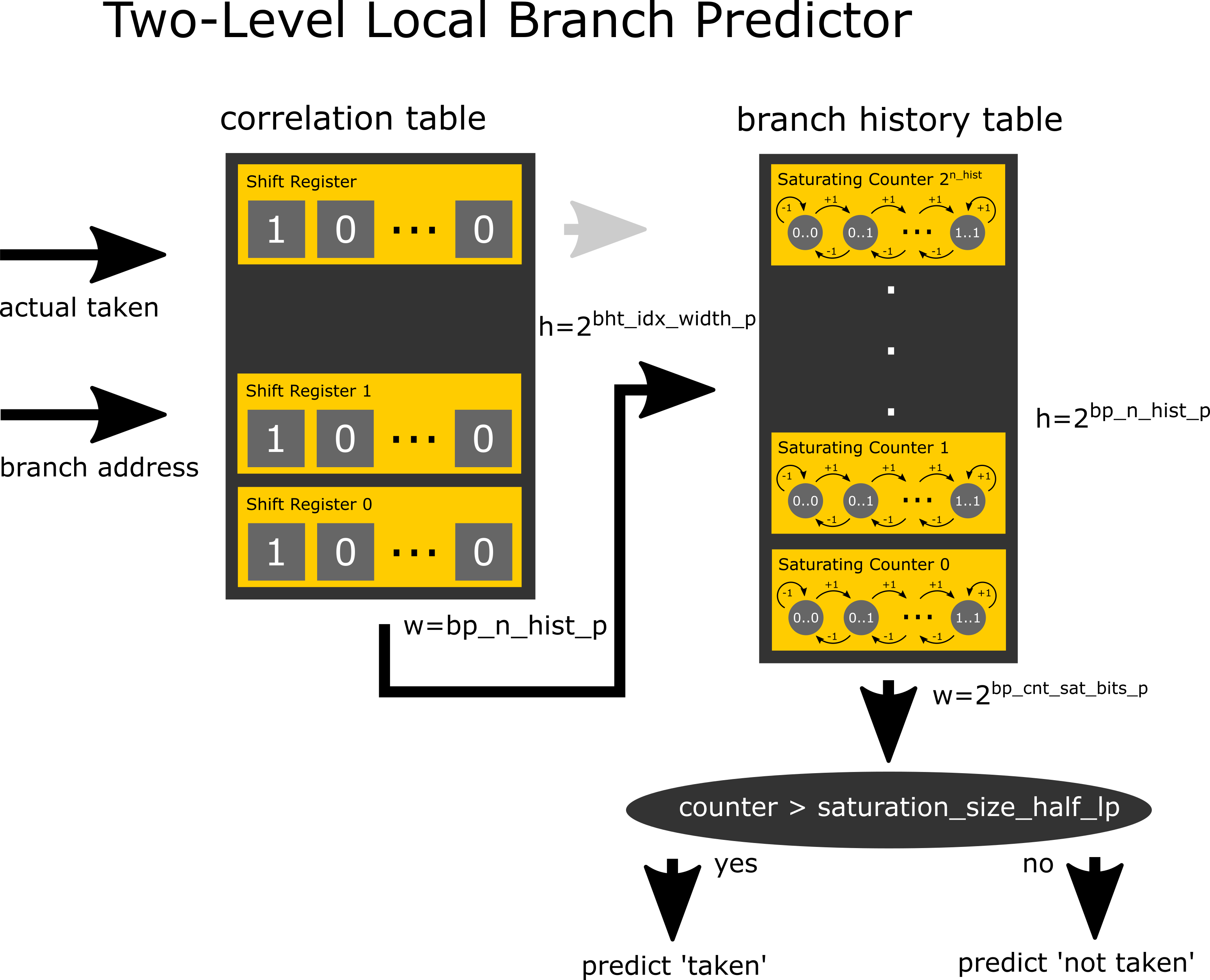
In order to solve the second issue of thoroughly test/simulate or design with a big amount of internal state, we decided to use cocotb, which allows us to co-simulate our RTL code (using verilator) and our model of the predictor written in python. Furthermore, we can use the traces from CBP-5, simulate them on both the RTL and python implementation and check if the output matches. This gives us high confidence of the correctness (considering the trace sizes). In addition to that, we can measure the actual accuracy (#correctly predicted/#all predictions) and do not have to rely on the indirect measure of the number of cycles. Furthermore, this process has been fully automated using travis-ci, such that after every push to the repo, the code is getting automatically re-tested (see travis-ci black-parrot-branch-predictor) To get a better understanding of the working principle, we illustrated the functionality below:
In this section, we will have a look at all branch predictor implementations, their functionality and performance.
Static branch predictors are very simple predictors used mostly used in the earliest processor designs. They do not rely on the branch history at runtime, but rather predict on the bases of the branch type.
The always not taken branch predictor is a static and ultra light-weight (area, power) branch predictor. Like the name already reveals, it simply predicts all branches as 'not taken'.
Accuracy: We expect this branch predictor to perform badly, and specifically worse than its always taken counterpart. The reasoning is that even if "if/else" branches might work in favour for either of them, most loops are implemented in the following general loop scheme works strongly in favour of the 'always taken' predictor:
C-Code:
x = 0;
while(x < 42){
    x++;
}
Assembly Version
        jmp     .L2
.L3:
        addl    $1, -4(%rbp)
.L2:
        cmpl    $41, -4(%rbp)
        jle     .L3
with x=-4(%rbp)
You note that the conditional jump jle is going to be 'taken' 42 times and only once 'not taken'.
Predictions per Cycle: Since there is no computation involved, the implementation should never end up on the critical path.
Area: The area usage should be close to zero.
Power: The power usage should be close to zero.
More detailed evaluations and the integration into black-parrot can be found:
The always taken branch predictor is a static and ultra light-weight (area, power) branch predictor. Like the name already reveals, it simply predicts all branches as 'taken'.
Accuracy: We expect this branch predictor to perform worse than the dynamical branch predictors, but better than its always not taken counterpart. The reasoning is that even if "if/else" branches might work in favour for either of them, most loops are implemented in the following general loop scheme works strongly in favour of the 'always taken' predictor:
C-Code:
x = 0;
while(x < 42){
    x++;
}
Assembly Version
        jmp     .L2
.L3:
        addl    $1, -4(%rbp)
.L2:
        cmpl    $41, -4(%rbp)
        jle     .L3
with x=-4(%rbp)
You note that the conditional jump jle is going to be 'taken' 42 times and only once 'not taken'.
Predictions per Cycle: Since there is no computation involved, the implementation should never end up on the critical path.
Area: The area usage should be close to zero.
Power: The power usage should be close to zero.
More detailed evaluations and the integration into black-parrot can be found:
Dynamic branch predictors not only rely on the branch type, but also incorporate information about branch outcomes during program execution.
Furthermore, the branch predictors we will see in this section can be generalized to consist of a branch history table (saturating counters representing the likelihood of taking/not taking the branch, with an update mechanism) and a hash function determining which counter to use.
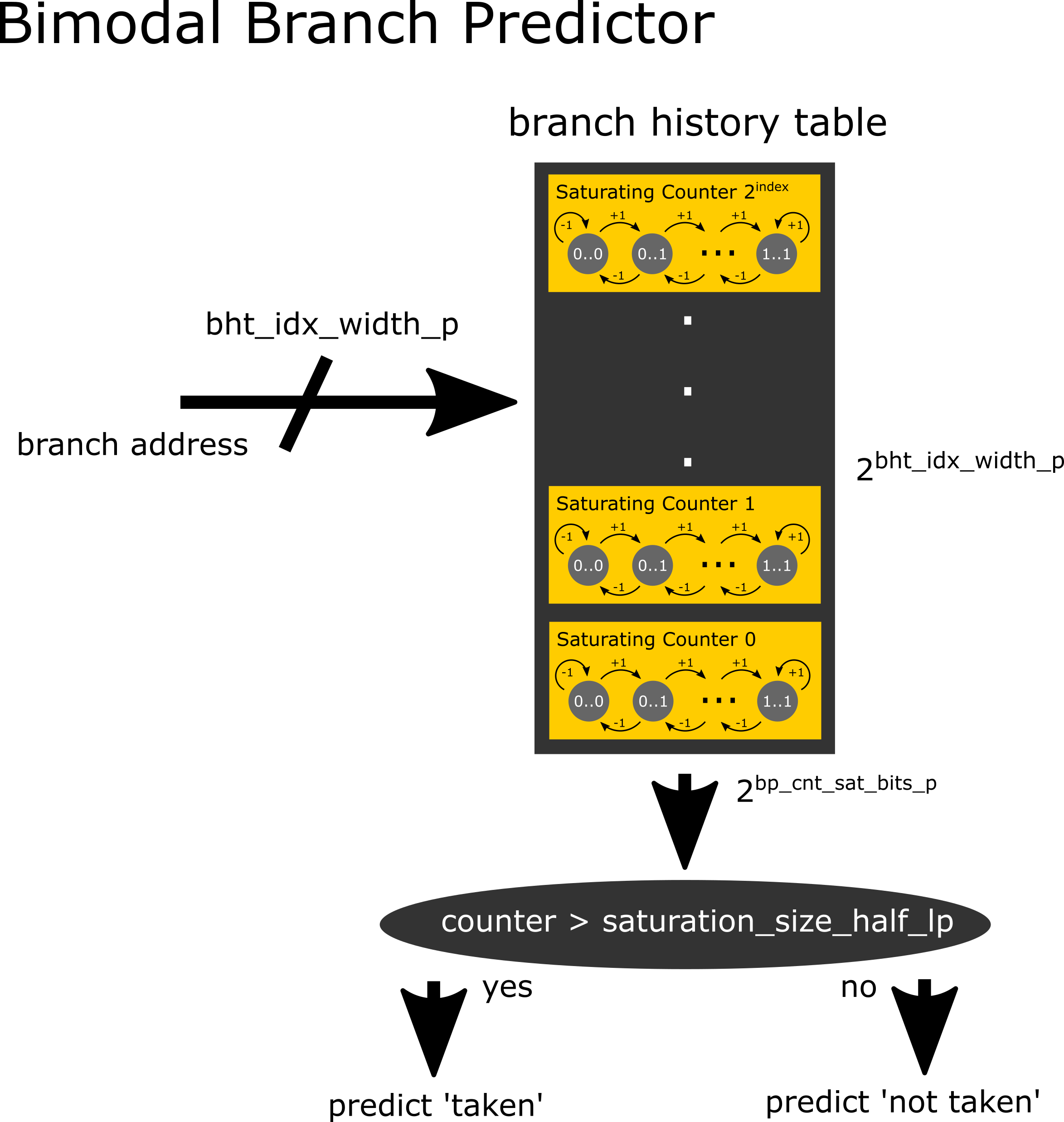
The bimodal branch predictor is a dynamic branch predictor that uses the lowest bht_indx_width_p bits as the hash function.
Accuracy: Since the bimodal branch predictor solely relies on the address bits for the hash, we expect this predictor to be good for workloads with very little correlation between sequential branches. For such workloads, this predictor should show better accuracy for smaller branch history table sizes, since this hash function does not spread very widely (and therefore we expect less collisions).
Area: Since the computational part of the module is rather small, we expect the area to grow linear with the size of the branch history table.
Power: Since the computational part of the module is rather small, we expect the power to scale linear with the size of the branch history table.
More detailed evaluations and the integration into black-parrot can be found:
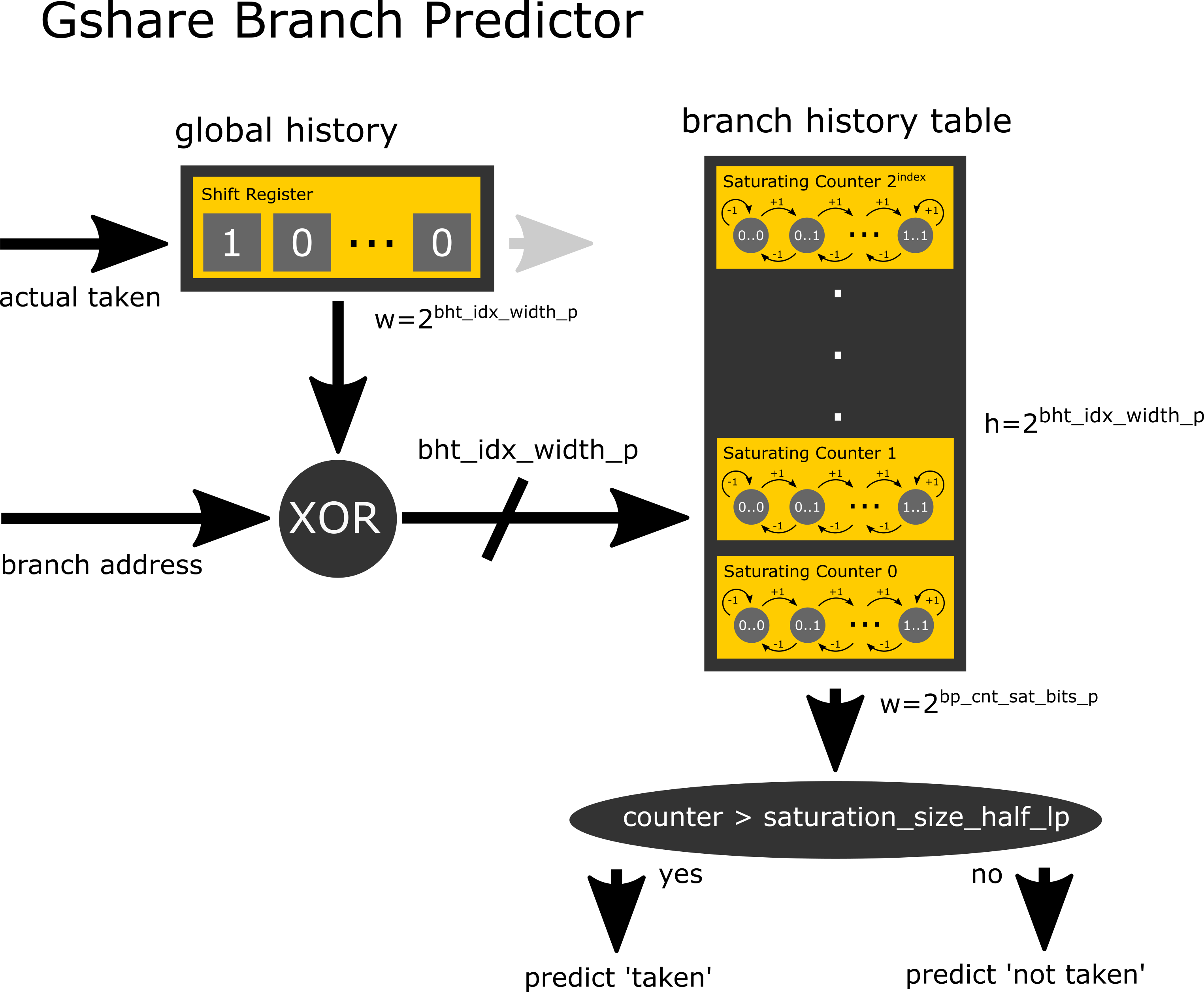
The gshare branch predictor is a dynamic branch predictor that uses the lowest bht_indx_width_p bits of the branch address
and the branch history xor-ed as its hash function.
Accuracy: Since applying bitwise xor over all available input information (branch address and branch history) should spread nicely over the whole hash image, we expect this predictor to perform very well on workloads with long branch correlation. Furthermore, because of the wide spread, we expect that this predictor can improve a lot over larger branch history table sizes.
Area: Since the computational part of the module is rather small, we expect the area to grow linear with the size of the branch history table plus the size of the branch history.
Power: Since the computational part of the module is rather small, we expect the power to scale linear with the size of the branch history table plus the size of the branch history.
Performance (backend flow):
| test case | instr/s |
|---|---|
| Towers | 75.65 |
| Vvadd | 56.24 |
| Median | 45.15 |
Power (backend flow):
| test case | mJ/s |
|---|---|
| Towers | 0.75 |
| Vvadd | 1 |
| Median | 1.586 |
Area (backend flow): 61448.6913 nm^2
More detailed evaluations and the integration into black-parrot can be found:
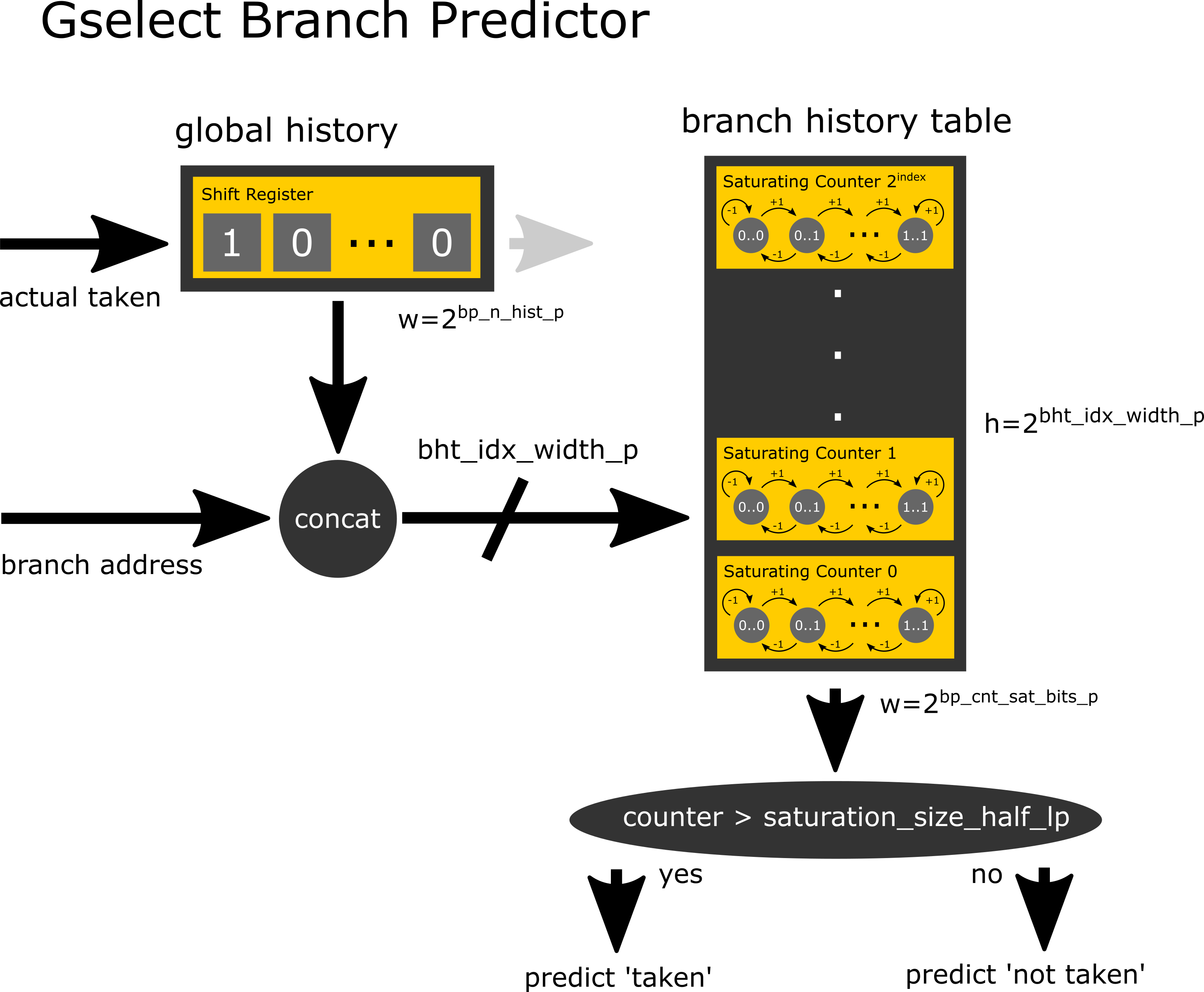
The gselect branch predictor is a dynamic branch predictor that uses the lowest bht_indx_width_p - bp_n_hist bits of
the address, concatenated with the bp_n_hist latest branch history bits as its hash function.
Accuracy: The gselect branch predictor is a trade-off between full spreading of the information (gshare) and only using the branch address (bimodal). We therefore expect the result of this predictor to be somewhere between the two others. In theory, in case of a workload that fits very well for the combination of history bits and address bits selected for this implementation, it could also outperform the other two.
Area: Since the computational part of the module is rather small, we expect the area to grow linear with the size of the branch history table plus the size of the branch history.
Power: Since the computational part of the module is rather small, we expect the power to scale linear with the size of the branch history table plus the size of the branch history.
Performance (backend flow):
| test case | instr/s |
|---|---|
| Towers | 80.45 |
| Vvadd | 72.84 |
| Median | 37.51 |
Power (backend flow):
| test case | mJ/s |
|---|---|
| Towers | 0.8589 |
| Vvadd | 0.8937 |
| Median | 1.802 |
Area (backend flow): 61044.9405 nm^2
More detailed evaluations and the integration into black-parrot can be found:
The tournament branch predictor is a dynamic branch predictor that uses a hybrid approach. One branch predictor uses the branch address only as a hash function, while the other one uses the branch history shift register only. In order to choose which of both predictions we should use, there is an additional saturating counter, the selector, which gives trust to either of them, depending on the correctness of their previous predictions.
Accuracy: While this branch prediction uses two branch predictors internally, it mostly gets the best result out of both words. We therefore expect this one to perform reasonably close to the maximum prediction accuracy of both internal branch predictors.
Area: Since the computational part of the module is rather small, we expect the area to grow linear with the size of the branch history tables plus the size of the branch history.
Power: Since the computational part of the module is rather small, we expect the power to scale linear with the size of the branch history tables plus the size of the branch history.
Performance (backend flow):
| test case | instr/s |
|---|---|
| Towers | 78.02 |
| Vvadd | 77.29 |
| Median | 39.38 |
Power (backend flow):
| test case | mJ/s |
|---|---|
| Towers | 0.77 |
| Vvadd | 0.7568 |
| Median | 1.508 |
Area (backend flow): 117722.4186 nm^2
More detailed evaluations and the integration into black-parrot can be found:
The two-level local branch predictor uses the indirection over a (potentially huge) correlation table consisting of branch address indexed branch histories. The history is then used as an index to the actual branch history table consisting of saturating counters.
Accuracy: Since this predictor basically stores all the information given to him (and uses it), it should outperform all others (with the grain of salt for using a lot more area/power).
Area: Since the computational part of the module is rather small, we expect the area to grow linear with the size of the correlation table plus the branch history table.
Power: Since the computational part of the module is rather small, we expect the power to scale linear with the size of the correlation table plus the branch history table.
Performance (backend flow):
| test case | instr/s |
|---|---|
| Towers | 81.04 |
| Vvadd | 80.38 |
| Median | 45.12 |
Power (backend flow):
| test case | mJ/s |
|---|---|
| Towers | 0.7959 |
| Vvadd | 0.78999 |
| Median | 1.427 |
Area (backend flow): 196948.6813 nm^2
More detailed evaluations and the integration into black-parrot can be found:
Neural branch predictors found their way into modern high-performance/high miss-prediction penalty CPU designs (i.e. AMD Ryzen, especially because of their ability to remember long history information without the necessity of exponential scale. But still, they are resource hungry and we have to carefully balance and reduce unnecessary functionality in order to make them feasible for the black-parrot RISC-V processor.
The Perceptron Algorithm is one of the most basic neural network algorithm. With limited latency and area/power budget, it is probably the most reasonable starting point for a neural branch predictor.
In order to further minimize the footprint, the model currently supports the following features:
- input: parameterized number of address index and branch history bits (bits/binary instead of floats)
- binary classification (branch taken/not taken)
- integer only data type (no float)
- single training round (aka single update of perceptron weights)
- single perceptron (another design choice could be to have multiple perceptrons, branch address indexed)
- fixed data width integers
This design is still under development. The current evaluations can be found:
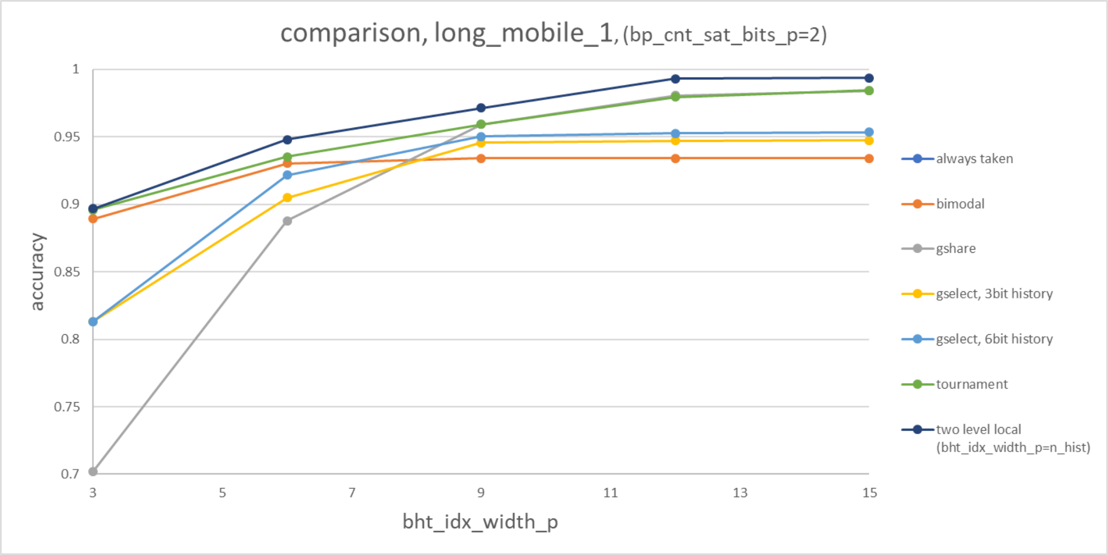
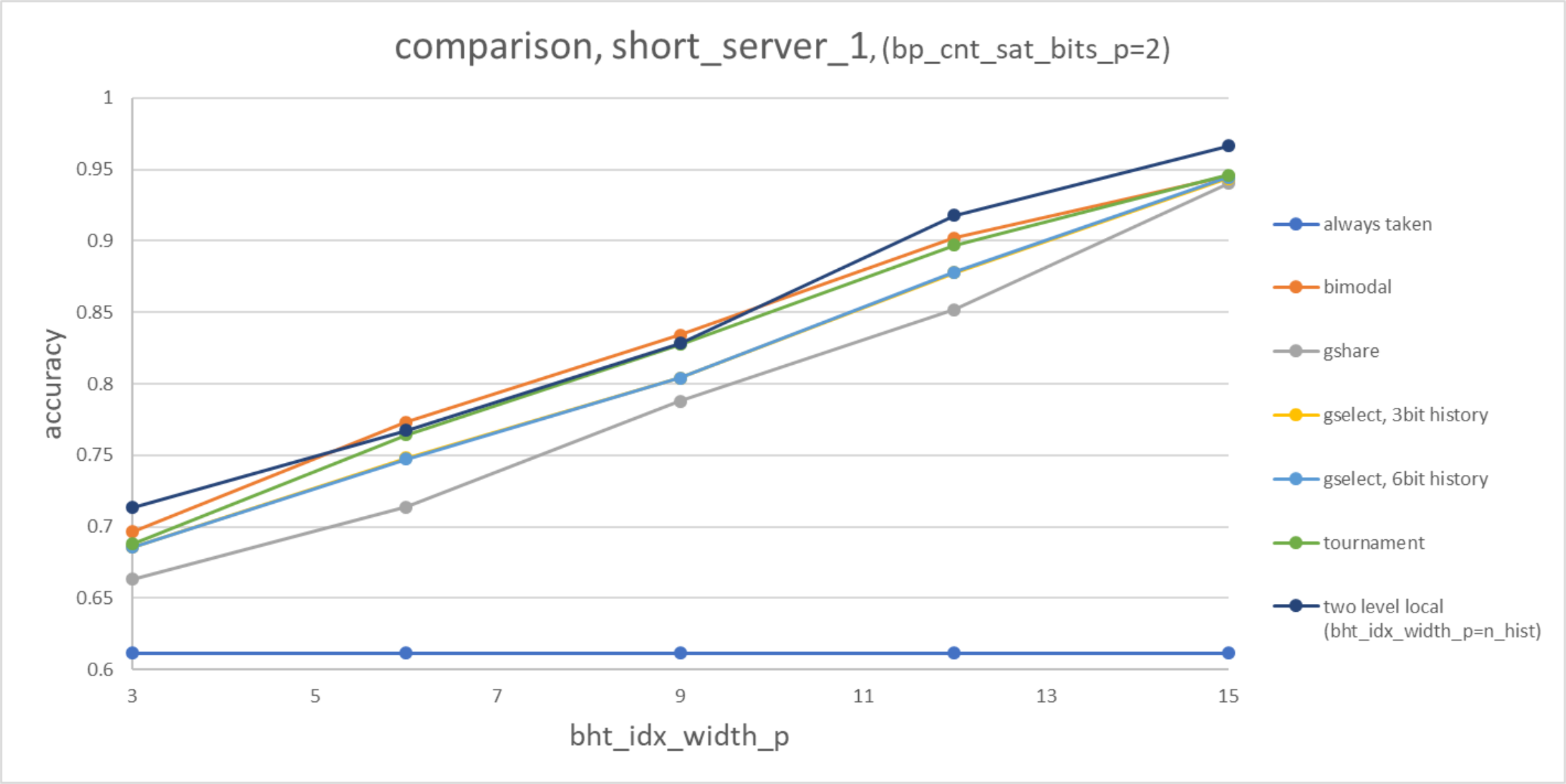
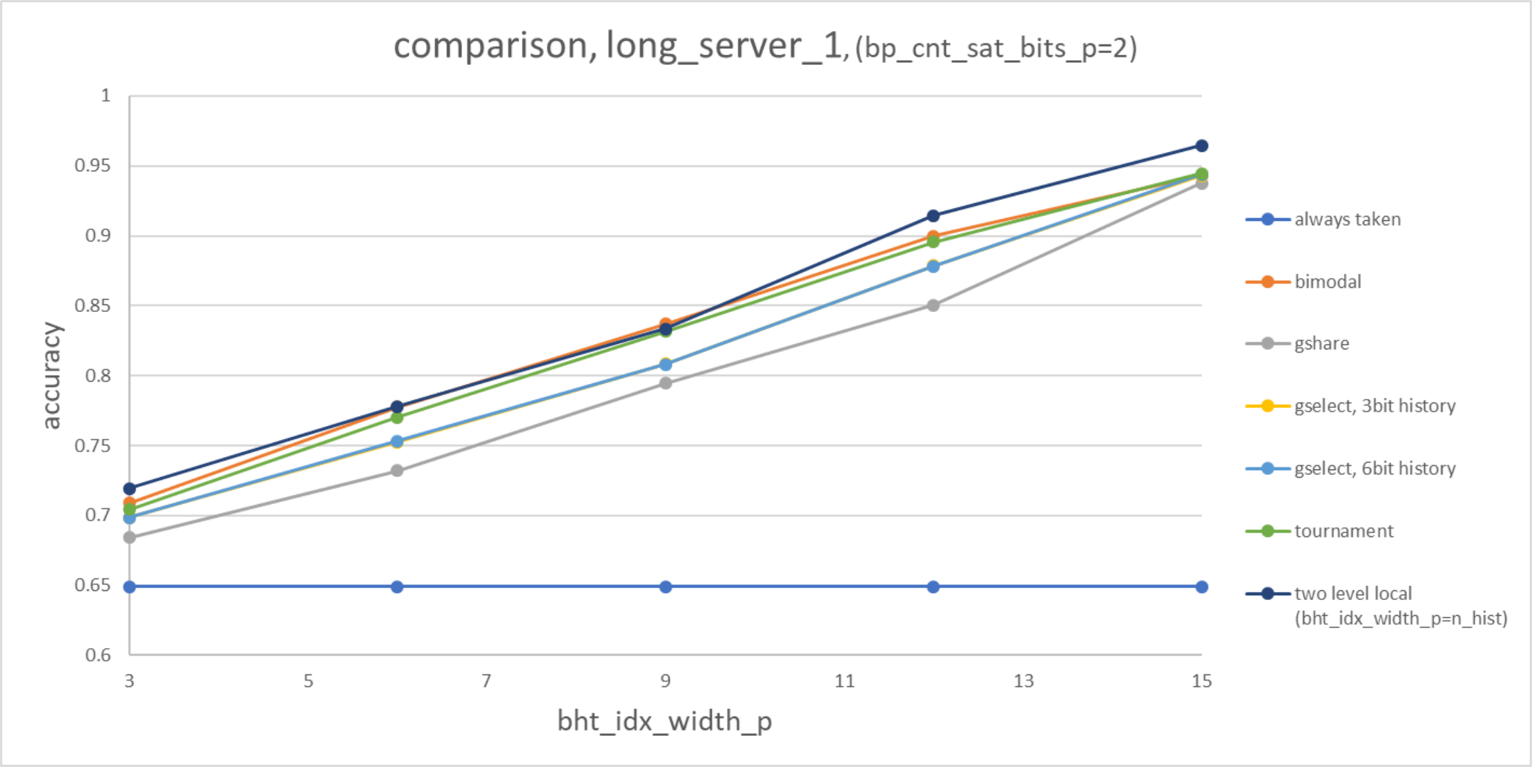
Generally, the problem of predicting the correct branch decision cannot be done previous to the evaluation of the conditional branch statement (in the presence of I/O and random number generators). Furthermore, there is usually a tight bound on the latency and resources (power/area) that are available for the implementation of such a predictor. Therefore, all the predictors use heuristics and are greedy, which means that most likely there does not exist the best predictor, but it is rather a balance between different trade-offs. These plots below provide insight into how much information each of the branch predictors is capable of storing, given different amounts of input information (in the form of branch history, address bits). It is important to note that the area and power requirements of different implementations might diverge significantly. For more information about that, refer to the theoretical power/area estimate and the findings from our backend flow.
always taken / always not taken:
- The conjecture about the performance increase of the 'always taken' over the 'always not taken' holds for all traces.
- The conjecture that the static branch predictor are more inaccurate than the dynamic branch predictors holds too.
bimodal: 3. We can see that the bimodal predictor has higher accuracy for small table sizes compared to gshare and gselect. For some of the traces the break-even point is earlier than for others. We therefore assume (unfortunately we cannot check this) that this is indeed due to the amount of correlation for the different test cases.
gshare: 4. We can see that the gshare predictor is worse for smaller table size, but because of its 'good spread', we see that it outperforms most of the others for larger table sizes.
gselect: 5. Depending on the trace, the accuracy is usually in between or close to the one from gshare and/or bimodal.
tournament: 6. Some traces show pretty nicely what we expected (i.e. long_mobile_1) and for others, the accuracy is close-by or slightly lower.
two-level local: 7. It outperforms all the other most of the time. Sometimes even very significantly.
Last but not least, a not so obvious conjecture was that the initial testing method did not add much of insight/relevance. With our own evaluation setup, we can e.g. distinguish quite clearly between the always taken and bimodal predictor performance, which was not possible before.
Furthermore, by running traces with over 10M branch instruction, we did not prove, but we know with high certainty, that either both RTL and the python model implementations are both correct or both wrong. But even if they would be wrong, according to Taylor's axiom, we are at least 10x faster in finding the bug! :)
Andreas:
Life is full of up and downs, and so is the choice of a good branch predictor. Doing the choice of your life within two weeks is probably a bit short-handed, but there is still one little beautiful idea that stand out of the mass. Taking two orthogonal implementations, and gluing them together using the very same basic, but well working building block (saturating counter) allows to (mostly) get the best of both words (see graph below: tournament vs bimodal/gshare/gselect).
In my opinion, we should use the tournament branch predictor, since this approach scales very well (upon changes of parameter bht_idx_width_p) with size, which is an important characteristic for the flexibility and re-usability approach of black-parrot (choosing the right parameters depending on the available power/area budget).
For this simplified power estimate model, we assume that the predictors power and area usage scales with its RAM size. We think that his is a reasonable assumption, since the remaining part of the predictors above has either a constant overhead or at least scales slower than the RAM.
Below you can see a table with logarithmic size axis that show how the branch history table scales.
We can conclude that the branch predictors, except the two-level local bp can e directly compared while we have to take the better accuracy of the two-level local pb with a grain of salt, due to its high cost in terms of area/power
- Change into the testbench_NAME directory
cd testbench_NAME - Execute the co-simulation by running
make(the trace file can be passed using:TRACE=long_server_1 make)
In order to execute all testbenches automatically, you can run make in the root directory of the repo.
- Run the co-simulation first. This should generate a file
dump.vcdin the testbench_NAME folder. - Open the waveform file using gtkwave
gtkwave dump.vcd
The following packages are required to run the simulation:
sudo apt install virtualenv build-essential python3-dev gtkwave verilator libboost-all-dev
To install all python packages, run the following command: pip3 install -r requirements.txt
We run our evaluation on the following system:
ubuntu 19.10 x86_64 kernel 5.3.0-40-genericpython v3.8cocotb v1.3.0verilator v4.020 2019-10-06gcc v9.2.1
The raw data we used for generating the plots can be found here
Unoptimized assembly code can be generated from C using: gcc -S CODE.c -O0. We added both C and assembly version
here
More information about the traces can be found on their official homepage. Our traces
are part of a large collection of training cases, which we converted using or modified bt9 reader to simple
traces of the form: branch_address taken \n. They can be found downloaded from here.
The bt9 conversion tool can be compiled using cd bt9_reader && make and used by executing ./bt9_reader INPUT_TRACE OUTPUT_FILE
We used the following four traces for the evaluation with test file sizes (#branches):
- short_mobile_1.trace: 16'662'268
- long_mobile_1.trace: 29'269'647
- short_server_1.trace: 230'692'528
- long_server_1.trace: 149'246'445
file: ee477-designs/toplevels/bp_single_softcore/tcl/filelist.tcl
replace "$BP_FE_DIR/src/v/bp_fe_bht.v" on line 163 with:
$BP_FE_DIR/src/v/bp_fe_bp.v
$BP_FE_DIR/src/v/bp_fe_bp_bimodal.v
$BP_FE_DIR/src/v/bp_fe_bp_gshare.v
$BP_FE_DIR/src/v/bp_fe_bp_gselect.v
Even though we tried to implement our branch predictor designs as generic as possible, we could still not incorporate all extra tweaks and tricks we found on the web.
We encourage people to contribute to this repo by adding additional testbenches. A few ideas for superior designs might be:
-
Perceptron Branch Predictor: The first version of the model is already implemented. We have to find a good balance between a good prediction rate and the complexity of the hardware (in terms of resources and critical path).
-
TAGE:
-
Furthermore, so far, we only used the branch address and branch history information for our branch predictions. There might be some headroom for improvement by applying additional heuristics such as looking at the type of branch instruction.
Any kind of feedback/issues or pull requests are welcome.
For moral support, you can also buy me a cup of coffee:
- https://github.com/black-parrot/black-parrot
- https://cocotb.readthedocs.io/en/latest/index.html
- https://www.veripool.org/wiki/verilator
- https://github.com/antmicro/cocotb-verilator-build
- https://web.engr.oregonstate.edu/~benl/Projects/branch_pred/#l3
- https://en.wikipedia.org/wiki/Branch_predictor#Local_branch_prediction
- http://people.cs.pitt.edu/~childers/CS2410/slides/lect-branch-prediction.pdf
- https://medium.com/@thomascountz/19-line-line-by-line-python-perceptron-b6f113b161f3

