Fitting the model from Gupta & Brody to human behavioral data. Based on https://codeocean.com/capsule/0617593/tree/v1.
By Anne Urai, 2022
conda create -n ssm_env
conda activate ssm_env
conda install cython
conda install seaborn
git clone https://github.com/lindermanlab/ssm.git
cd ssm
pip install -e .
Following simple linear dynamical system (LDS) is used to disentangle slow drifts from systematic updating:
-
$X_t$ is a latent process (i.e. the slow drift) and follows an AR(1) process. -
$U_t$ is a matrix and contains input variables that can influence the latent process (none, in our case) -
$b$ is a bias, or intercept -
$Y_t$ represents the (observed) emissions -
$U_t$ is a matrix and contains input variables that can influence the emissions- stimulus strenght, previous confidence, previous response...
-
$d$ is a bias, or intercept
With these parameters the model can be rewritten as:
with
We simulated 20 datasets with a varying number of trials. Model was fitted with EM procedure and 100 iterations. Simulations showed good parameter recovery, even for datasets with low number of trials (n=500). However, sigma seems hard to estimate. In addition, we see an interesting trade-off between sigma and C. The lower sigma, the higher C get, and vice versa.

20 datasets were simulated with 500 trials each. Number of iterations does not seem to play a role for most parameters. Also here we see a trade-off between sigma and C (albeit less clear due to scaling).

gonna improve these simulations and plots later
If we simulate data with slow drifts and systematic updating of previous response, confidence, sign evidence and absolute evidence we see a nice recovery when the model fits both slow drifts and systematic updating. Especially given the fact that this is only with 500 trials (still going to check how this is for more trials)

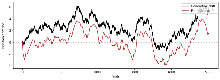
If we simulate data with only slow drifts, and the model is only allowed to estimate systematic updating, then we see these apparent updating strategies (and an underestimation of the ground truth perceptual sensitivity). This replicates the earlier simulations in R, and the simulations by Lak et al, Mendonca et al, Gupta & Brody.

If we fit the model to real data (beehives task), treating all participants as one 'super-participant', we see that the model converged nicely.

This is the estimated slow drift (sudden jumps probably due to switches over participants?)

These are the estimates for the systematic updating. In this order: sensitivity, prev resp, prev conf, prevresp_prevconf, prev sign evidence, prev abs evidence, prevsign_prevabsevi. Although it seems that these values are rather small, plotting and testing is needed to see there is still an effect.

- Why is a random walk imposed on the latent process instead of fitting the AR(1) coefficient?
- Now
A = 1andCis fitted
- Now
- Would the estimation work with only 500 trial per participant? Or would a switching LDS where the drifting criterion jumps between observers be better? We could confirm by checking if the estimated state transitions occur where the data of a new participant starts.
- How is the analytical computation of sigma done? And why analytical?
- How to interpret
C,sigma, and their trade-off mechanism?

-
Why is the slow drift in data simulation mean centered?
- If we don't center we get something like this:
- If we don't center we get something like this:
-
Why is
estDriftcomputed by multiplyingCs? Sort of scaling to compensate for A = 1?

- what is the minimum number of trials needed to retrieve slow drift + history weights?
- How does this depend on the size of the noise sigma?
- is there a numerical determinant of ELBO convergence? -> no, have to inspect visually
- how many
num_iterdo we need? - how do
predEmissionscompare to binary choices? - nice to have: printing function (with explanation of parameters)?
- does it matter that some trials are deleted due to timed-out responses?
- what if simulated drift has a AR coef lower than .9995, can the model still account for this given that a random walk being imposed?
- answer: with our trial counts, can we even expect to get good fits?
- try simulations with data-ish parameters
- add confidence-scaling (use previous R simulations and fit with ntrials = 500)
- fit to real data from Beehives or Squircles task
- correlate single-subject beta's with GLM weights
- compare confidence-betas with R output
- and with and without fixing sigma at 0
- concatenate all trials across participants, then fit with a switching LDS where the drifting criterion jumps between observers
- what if the frequency of the slow drift wave changes over time? eg faster oscillations over time, problem because we only fit one AR coef?
- how does the fitting behave if sigma is not estimated analytically?
- design matrix predictors
- plotting psychometric functions
- hypothesis testing for systematic updating
- fit on squircles dataset