| author | beastversion | tracerversion | level | title |
|---|---|---|---|---|
David A. Rasmussen, Joëlle Barido-Sottani |
2.6.0+ |
1.6.0 |
Beginner |
Troubleshooting |
The primary goal of most phylogenetic analyses in BEAST is to infer the posterior distribution of trees and associated model parameters using Markov chain Monte Carlo (MCMC) sampling. In this tutorial, we will learn how to analyze the output of a MCMC analysis in BEAST using Tracer. This program allows us to easily visualize BEAST's output and summarize results. As we will see, we can also use Tracer to troubleshoot some of the most common MCMC problems encountered in BEAST.
While BEAST's MCMC algorithm is fairly well optimised for phylogenetic inference, problems can arise, especially as the complexity of our data and models increase. A MCMC run may not converge on a stationary target distribution. More commonly, a run might converge but mix poorly - meaning our samples from the posterior are highly autocorrelated and therefore not independent. In these cases, it is often necessary to tune the performance of the MCMC algorithm.
BEAST2 (http://www.beast2.org) is a free software package for Bayesian evolutionary analysis of molecular sequences using MCMC and strictly oriented toward inference using rooted, time-measured phylogenetic trees. This tutorial is written for BEAST v{{ page.beastversion }} {% cite BEAST2book2014 --file Troubleshooting/master-refs %}.
BEAUti2 is a graphical user interface tool for generating BEAST2 XML configuration files.
Both BEAST2 and BEAUti2 are Java programs, which means that the exact same code runs on all platforms. For us it simply means that the interface will be the same on all platforms. The screenshots used in this tutorial are taken on a Mac OS X computer; however, both programs will have the same layout and functionality on both Windows and Linux. BEAUti2 is provided as a part of the BEAST2 package so you do not need to install it separately.
Tracer (http://tree.bio.ed.ac.uk/software/tracer) is used to summarise the posterior estimates of the various parameters sampled by the Markov Chain. This program can be used for visual inspection and to assess convergence. It helps to quickly view median estimates and 95% highest posterior density intervals of the parameters, and calculates the effective sample sizes (ESS) of parameters. It can also be used to investigate potential parameter correlations. We will be using Tracer v{{ page.tracerversion }}.
In this part of the tutorial, we will see several issues which can prevent a BEAST2 inference from even starting, and demonstrate how to fix them.
All examples in this section are inspired by real issues encountered during the analysis of the convergent evolution of true crabs {% cite Wolfe2022 --file Troubleshooting/master-refs %}. The dataset used is composed of sequences for 344 extant species of the infraorder Brachyura, in addition to fossil calibrations or fossil samples for this clade. Note that the runs presented here have been simplified from the original, in particular many of the alignment partitions used in the original analysis have been removed.
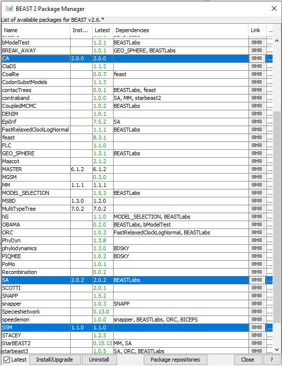
The following packages are required to run the examples: SA, CA, SSM.
Figure 1: Finding the BEAST2 Package Manager.Launch BEAUti, then open the BEAST2 Package Manager by navigating to File > Manage Packages. (Figure 1)
Figure 2: The BEAST2 Package Manager.Install the CA, SA and SSM packages by selecting them and clicking the Install/Upgrade button. (Figure 2)
BEAUti needs to be closed for the newly installed packages to be loaded properly.
Close the BEAST2 Package Manager and BEAUti.
Figure 3: Error message in BEAST2.Download the BEAST input file
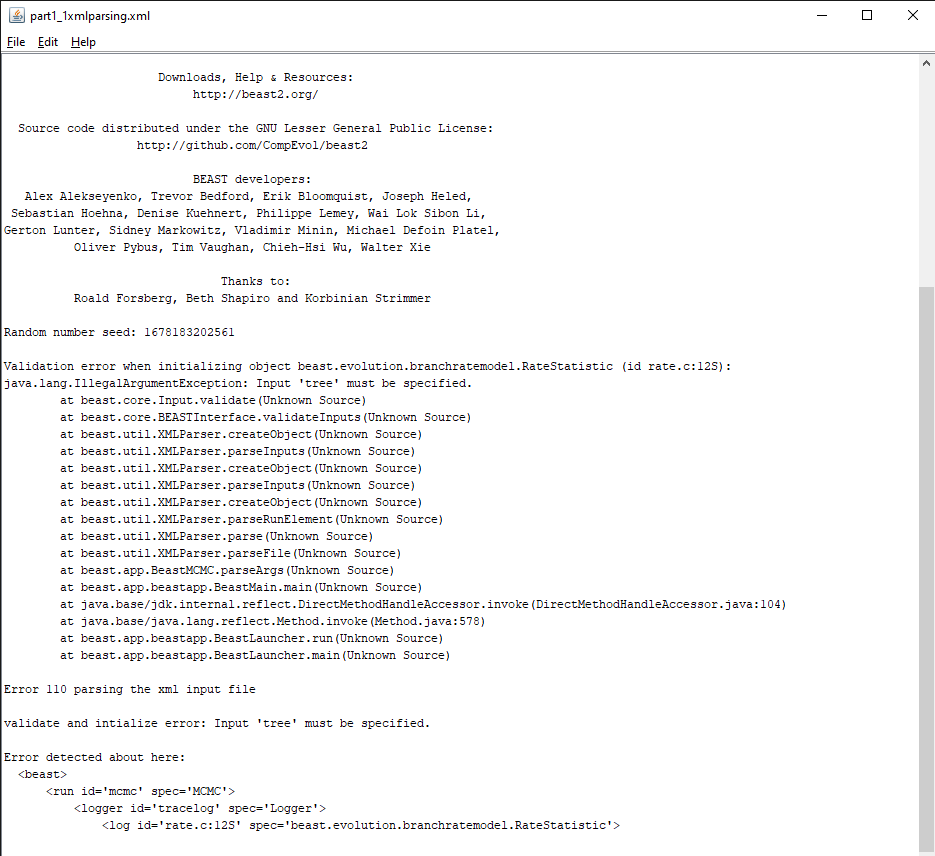
part1_xmlparsing.xmlandpart1_1xmlparsing_working.xml. Open BEAST2 and select the filepart1_xmlparsing.xmlas input file. Start the run with the Run button. You should get an error message, as shown in Figure 3.
Here the run failed to start because the XML configuration file could not be parsed, as explained by the error message Error 110 parsing the xml input file. Thankfully the error message tells us exactly where the error happened () and what is the issue (Input 'tree' must be specified.). If we open the part1_xmlparsing.xml file and look for rate.c:12S, we can see that line 1297 corresponds to the error message and reads as follows:
<log id="rate.c:12S" spec="beast.evolution.branchratemodel.RateStatistic" branchratemodel="@RelaxedClock.c:12S"/>By comparing to a previous (working) analysis in the file part1_1xmlparsing_working.xml, we can see that the correct configuration should be (line 497):
<log id="rate.c:12S" spec="beast.evolution.branchratemodel.RateStatistic" branchratemodel="@RelaxedClock.c:12S" tree="@Tree.t:concat"/>As the error message told us, the tree element of the configuration is missing in the non-working XML file. Putting it back allows us to start the run.
Open the file
part1_xmlparsing.xmlin a text editor. Modify line 1297 of the file to add thetree="@Tree.t:concat"element. Save the file aspart1_xmlparsing_fixed.xml. Open BEAST2 and select the filepart1_xmlparsing_fixed.xmlas input file. Start the run with the Run button. Now it works!
XML parsing errors usually occur when the XML file has been manually edited and parts of the configuration have been accidentally deleted or modified. This is why it's important to always keep a copy of the original XML when making manual edits, as this provides an easy way to check the correct configuration. If an XML parsing error occurs in a file which was generated entirely through BEAUti, then this is likely a BEAUti bug and should be reported to the development team.
Figure 4: Another error message in BEAST2.Download the BEAST input file
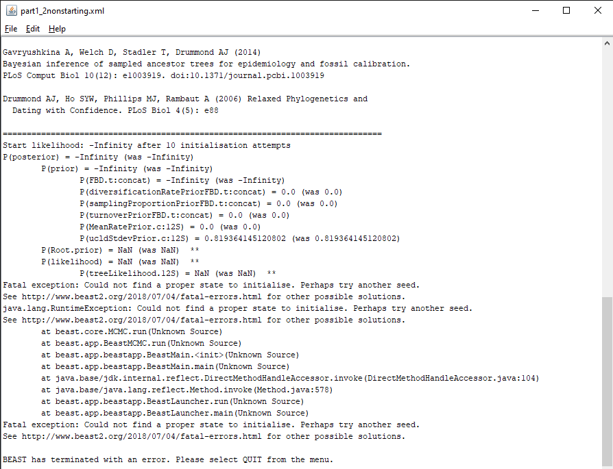
part1_2nonstarting.xml. Open BEAST2 and select the filepart1_2nonstarting.xmlas input file. Start the run with the Run button. You should get an error message, as shown in Figure 4.
In this situation, the inference failed to start because a good initial state could not be found, as explained by the error message (Fatal exception: Could not find a proper state to initialise.). This issue is much more complex to diagnose than the previous one, as it can be caused by many different parts of the analysis configuration. However, as above the error message provides some information on the source of the problem, as it details the probability of all the components of the analysis. The message reads P(FBD.t:concat) = -Infinity, showing that the issue likely appears in the calculation of the FBD likelihood. The FBD prior is a tree prior, and depends on the tree as well as several other parameters, so there are several possible causes for the calculation issue:
- a bug in the likelihood calculation itself: BEAST2 packages can contain calculation issues which have been undetected so far (especially if they only appear in very specific circumstances), in which case they should be reported to the development team. However, this is unlikely in our case, as the FBD model has been extensively used without issue in previous analyses, and our analysis setup is similar to previous analyses.
- an issue with the initial tree: the inference will not start if the provided initial tree is impossible under the specified tree model or doesn't match with the provided MRCA constraints. By default, most analyses use a random tree simulated by the inference, which will fulfill all constraints. However, with more complex models or constraints, the simulation process can fail to find a good tree, in which case a valid starting tree needs to be provided by the user.
- an issue with the initial values of the parameters: if the initial values set in the analysis are very far from plausible, the resulting likelihood of the model will be extremely small, which gets recorded as -Infinity by BEAST2.
To inspect the starting values and find the issue, we will first load the file into BEAUti.
Open BEAUti and load in the
part1_2nonstarting.xmlfile by navigating to File > Load.
The starting tree can be found in the Starting tree panel, which is hidden by default.
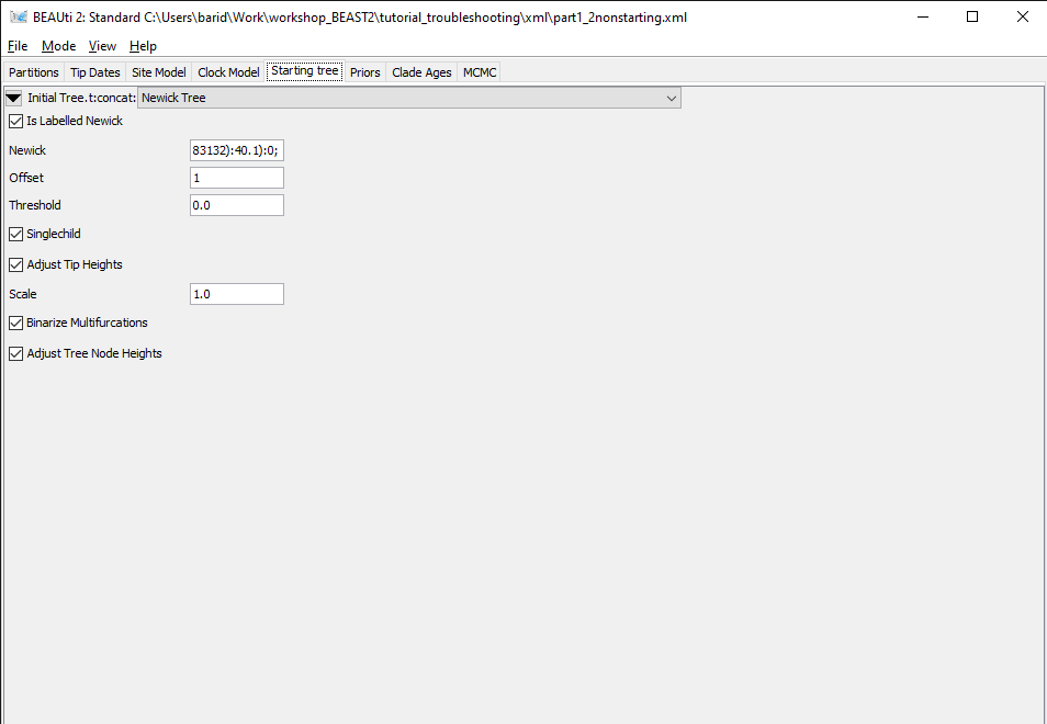
Figure 5: Starting tree panel.Open the Starting tree panel by navigating to View > Show Starting tree panel. Switch to the Starting tree panel.
As we can see in Figure 5, the initial tree in this analysis is set to a Newick tree, chosen by the user. The Newick box gives the full Newick string, which we could use to inspect the tree in an other program. This string can also be copied directly from the XML file. First, we will check if this tree is compatible with the tree constraints set in the Priors panel.
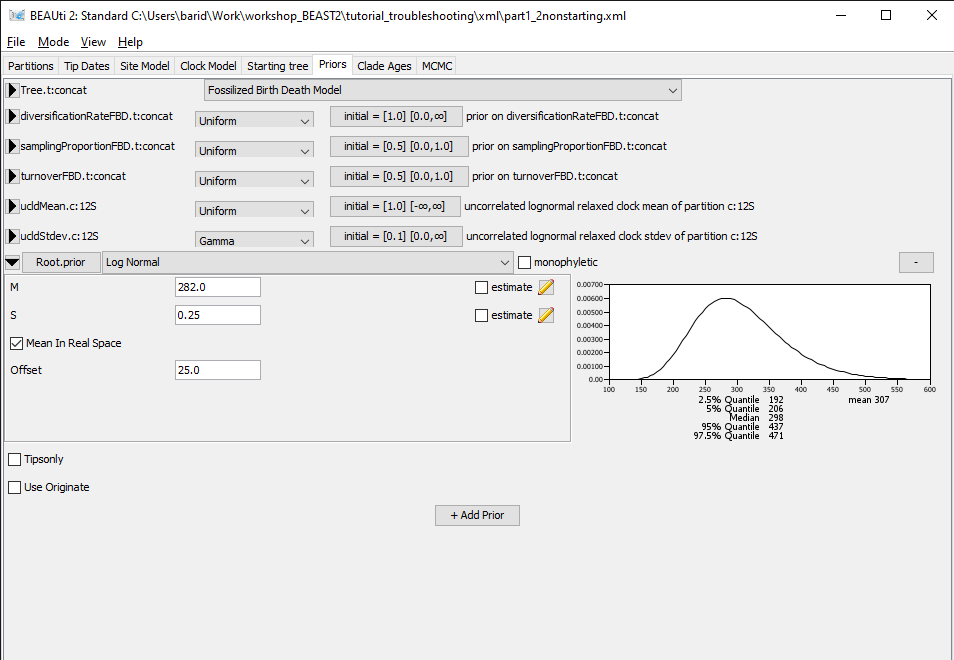
Figure 6: Priors panel showing the root prior.Switch to the Priors panel. Click on the arrow left of the Root.prior to see the details of this prior (Figure 6).
The only constraint set on the tree is a prior on the age of the root, which we can see in the Priors panel. By checking the details, we can see that this is a wide lognormal prior, with the 5% quantile of the prior at 206 Ma and the 95% quantile at 437 Ma. Let's import our starting tree in Icytree to check if the root age is compatible with the prior.
Open Icytree (https://icytree.org/) in a web browser. Copy the Newick string from the Starting tree panel or from the XML file. Paste the string into a blank text file and save it as
starting.tre. Drag and drop thestarting.trefile into Icytree.
By hovering over the root node of the starting tree, we can see that its age is set to 305.91 Ma, which is consistent with the root prior set in the analysis.
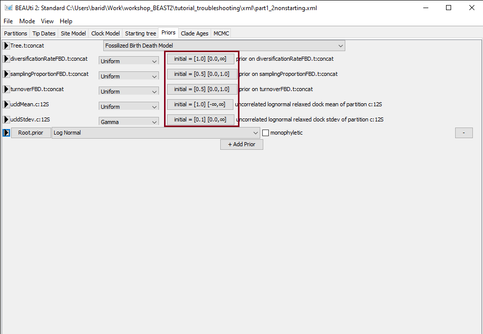
Next, we will inspect the starting values of the parameters of the FBD model, found in the Priors panel in BEAUti. The FBD model has 3 parameters: the diversification rate, the turnover and the sampling proportion. For each parameter, the starting value is shown in the box to the right, as initial = [x] [min, max] (Figure 7). Here x indicates the starting value and min and max the range of possible values for the corresponding parameter. Thus we can see that the initial diversification rate is 1.0, the initial sampling proportion is 0.5 and the initial turnover is 0.5. These are the default values for these parameters, but they may not be adapted to all datasets. In particular, a diversification rate of 1.0/My is a very high value - since our starting tree is 300 My old, it means that we would expect about exp(300 x 1.0) = 2 x 10^130 extant species. Having a very implausible starting value for the diversification rate could explain the failure we observed earlier when calculating the likelihood of the FBD model, so we will change it to a more realistic value of 0.01.
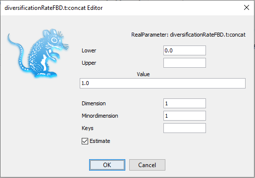
Figure 7: Initial values in the Priors panel.Figure 8: Changing the initial value.In the Priors panel, click on the initial = [1.0] box right of the diversificationRateFBD parameter. Change the initial value in the Value box to 0.01 (Figure 8). Click on OK to close the box. Save the updated configuration as
part1_2nonstarting_fixed.xmlby navigating to File > Save As. Open BEAST2 and selectpart1_2nonstarting_fixed.xmlas the input file. Start the run with the Run button. It works now!
In this part of the tutorial, we will consider a relatively simple example where we would like to infer a phylogeny and evolutionary parameters from a small alignment of sequences. Our job will be to work together to increase the efficiency of the MCMC so we can get the analysis to converge...
To get started, I have generated a XML file that we can run our phylogenetic analysis in BEAST.
Download the first BEAST input file
part2_tutorial_run1.xml
The XML contains an alignment of 36 randomly simulated DNA sequences.
While we can open the XML file in any standard text editor, BEAUTi offers an easy way to inspect the different elements of the analysis:
Open BEAUti and load in the
part2_tutorial_run1.xmlfile by navigating to File > Load.
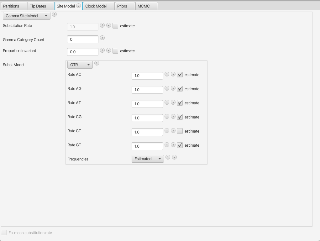
By navigating between the different tabs at the top of the application window, we can inspect the data and each element of the analysis. For example, in the Site Model panel, we can see that we are fitting a GTR substitution model with no gamma rate heterogeneity (Figure 9).
Figure 9: The Site Model panel in BEAUTiWe are now ready to run our first analysis in BEAST.
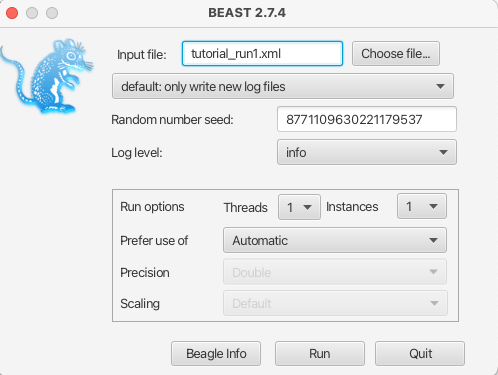
Figure 10: Running BEAST with the specified XML configuration file.Open BEAST and choose
part2_tutorial_run1.xmlas the BEAST XML file. Then click Run.
Since we are only running 200,000 iterations, the MCMC should finish running in under 30 seconds.
Open Tracer and navigate to File > Import Trace File, then open
part2_tutorial_run1.log
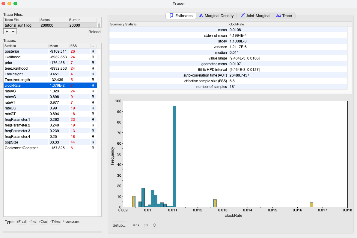
The results of your run will look similar, but not necessarily identical, to my results shown in Figure 10.
Tracer allows us to quickly visualize BEAST's MCMC output in order to check performance and see our parameter estimates. On the left there is a panel where all model parameters are listed along with their mean posterior estimates and Effective Sample Size (ESS). Recall that the ESS tells us how many pseudo-independent samples we have from the posterior, so the higher the better. Here, we can see that the ESS is low for all parameters, indicating that we do not yet have a good estimate of the posterior distribution.
By selecting a parameter in the left panel and then clicking on the Trace tab, we can see how the MCMC explored parameter space (Figure 11). For the clockRate parameter for instance, we see that the chain quickly converged to a value of about 0.01 (the true value used to simulate the sequence data), but mixing was poor, hence the low ESS.
Figure 11: Trace plot of the clock rate parameterWe can also see our posterior estimates for each parameter by clicking on the Estimates tab while highlighting the desired parameter in the left panel. This provides us with various summary statistics and a frequency histogram representing our estimate of the posterior distribution constructed from our MCMC samples. For the clockRate parameter, we can see that our estimate of the posterior is extremely rough, again because we have so few uncorrelated samples from the posterior (Figure 12).
Figure 12: Posterior estimates of the clock rate parameter in Tracer.By checking the ESS, trace plots and parameter estimates, we got the picture that none of our parameters in Run 1 mixed well. In this case, the simplest thing to try is to rerun the MCMC for more iterations.
Load the
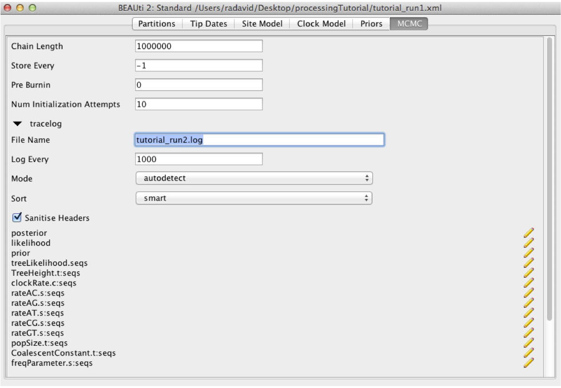
part2_tutorial_run1.xmlback into BEAUti using File > Load. Navigate to the MCMC panel and increase the chain length to 1 million. You may also want to change the file name for the log file topart2_tutorial_run2.logand topart2_tutorial_run2.treesfor the tree file so we do not overwrite our previous results. When done, navigate File > Save As and save aspart2_tutorial_run2.xml.
Figure 13: Increasing the chain length in BEAUTiRun the
part2_tutorial_run2.xmlfile in BEAST as we did before. When done, open thepart2_tutorial_run2.login Tracer.
Looking at the MCMC output in Tracer, we see that that increasing the chain length did help some (Figure 14). The ESS values are higher and the traces look better, but still not great. In the next section, we will continue to focus on the clockRate parameter because it still has a low ESS and appears to mix especially poorly.
Figure 14: Trace plot of the clock rate parameterIf one parameter in particular is not converging or mixing well, we can try to tweak that parameter's operator(s). Remember that BEAST's operators control what new parameter values are proposed at each MCMC iteration and how these proposals are made (i.e. the proposal distribution). Since the clockRate parameter was not mixing well in Run 2, we will try increasing the frequency at which new clockRates are proposed.
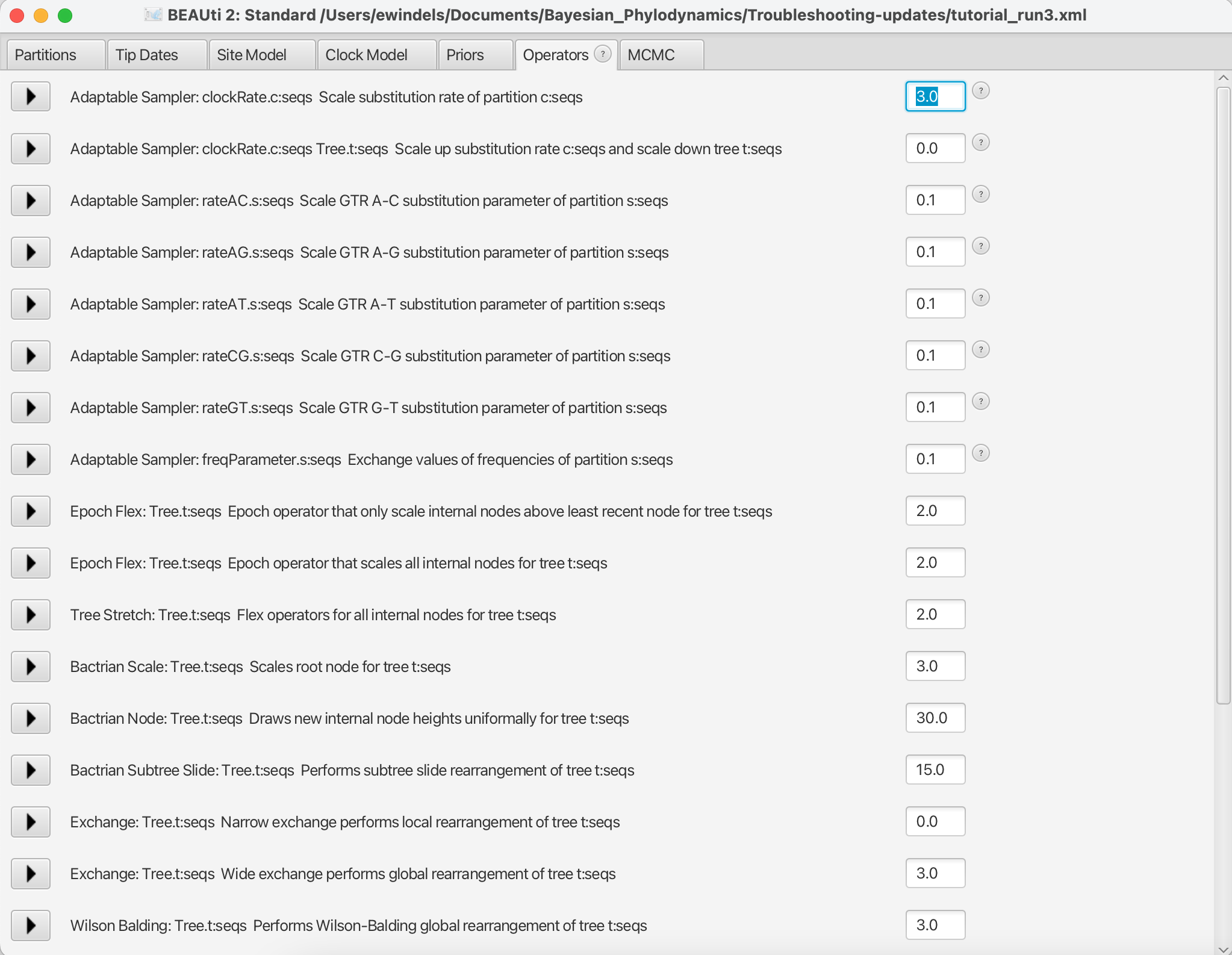
Figure 15: The Operators panel in BEAUTiLoad the
part2_tutorial_run2.xmlback into BEAUti and selectView > Show Operatorspanel. This will bring up a new panel showing all the operators in use (Figure 15). Click on the black triangle next toScale:clockRate. In the menu that drops down, check Optimise. In the box to the right ofScale.clockRate, change the value from 0.1 to 3.0. Now navigate to the MCMC panel and change the file name for the log file topart2_tutorial_run3.logand the tree file topart2_tutorial_run3.trees. When done, save aspart2_tutorial_run3.xml.
So, what just happened? We told BEAST to try to automatically optimise the scale operator on the clockRate, which moves the parameter value up or down. Note that by default, operators are automatically optimised in BEAST, but for the purposes of this tutorial I turned off auto-optimization to get especially bad mixing. We also increased the weight on this scale operator so that new clockRates will be proposed more often in the MCMC. Going from a weight of 0.1 to 3.0 means that new proposals for that parameter will be made thirty times as often, but the frequency at which a given operator is called depends on the weights given to other operators. So if there are parameters with very high ESS values, we may want to reallocate weight on their operators to operators on less well mixing parameters. For fun, you may want to guess what each operator in the Operators panel is doing.
Run the
part2_tutorial_run3.xmlin BEAST and then open thepart2_tutorial_run3.login Tracer.
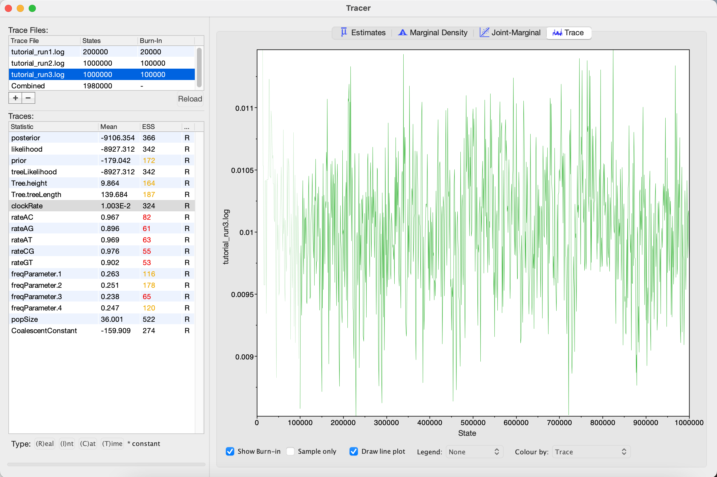
We can see that optimizing the operator dramatically improves mixing for the clockRate (Figure 16). But there is still room for improvement.
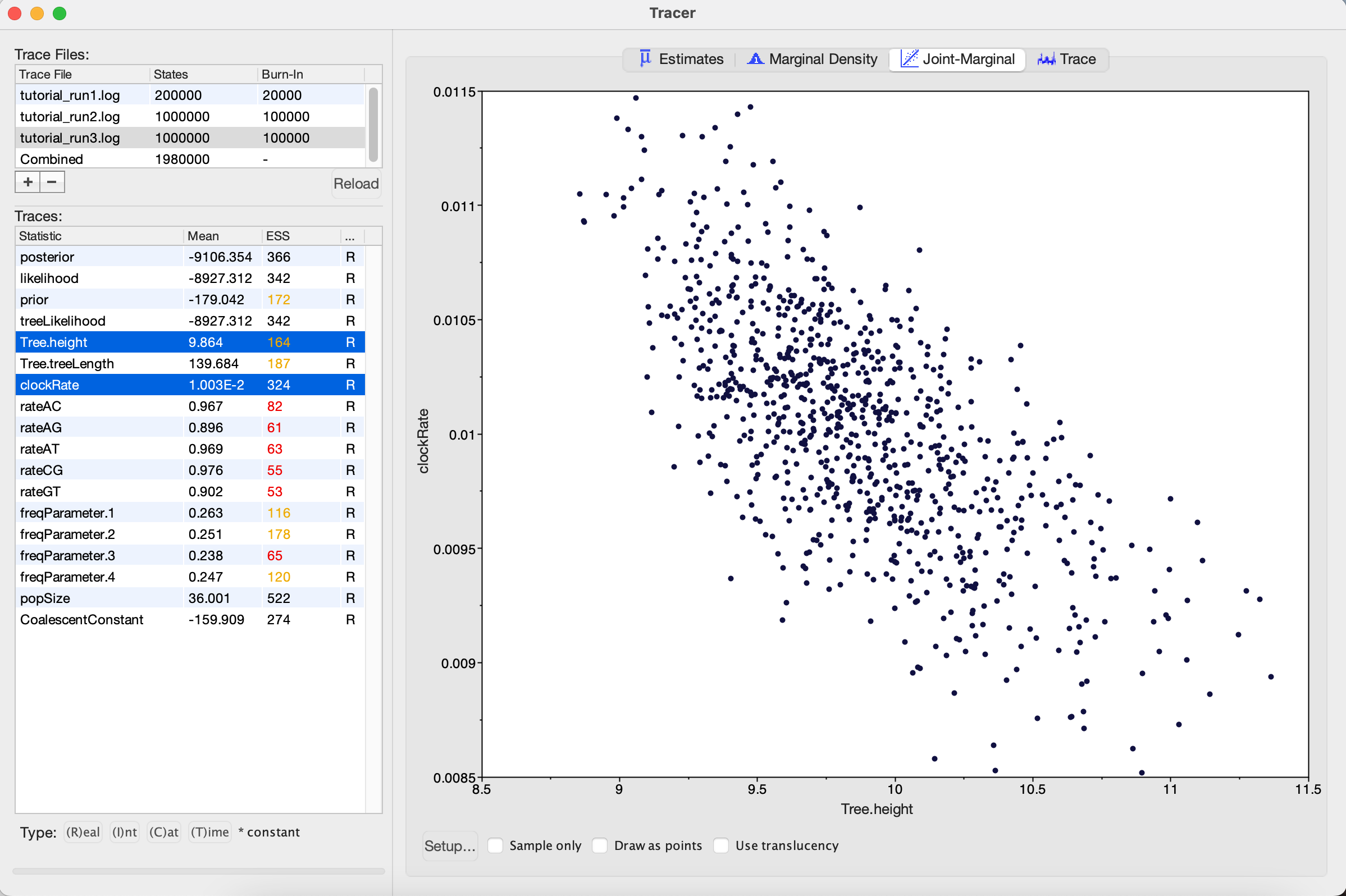
Figure 16: Trace plot of the clock rate parameterOne thing to keep in mind is that BEAST is using MCMC to explore a multidimensional parameter space, and poor mixing in one dimension can be caused by poor mixing in another dimension. This often arises because two parameters are highly correlated. We can identify these correlations in Tracer by visualizing the joint distribution of a pair of parameters together. To do this, select one parameter in the left panel and then, while holding the command key (Mac) or control key (Windows), select another. Then click on the Joint-Marginal tab at the top. Looking at the pairwise joint distribution for TreeHeight and clockRate, we see that these two parameters are highly negatively correlated (Figure 17). We therefore may want to add an operator that updates these parameters together to more efficiently explore their parameter space.
Figure 17: Joint posterior distribution of the tree height and clock rateThe easiest way to improve MCMC performance when two parameters are highly negatively correlated is to add an UpDown operator. This operator scales one parameter up while scaling the other parameter down. If two parameters are highly positively correlated we can also use this operator to scale both parameters in the same direction, up or down.
Load the
part2_tutorial_run3.xmlback into BEAUti and selectView > Show Operatorspanel. Click on the black triangle next to UpDown clockRate. In the menu that drops down, check Optimise. In the box to the right, change the weight on the UpDown operator from 0.0 to 3.0. In the MCMC panel, change the file name for the log file topart2_tutorial_run4.logand the tree file topart2_tutorial_run4.trees. When done, save as part2_tutorial_run4.xml`.
We just added an UpDown operator on the clockRate and the TreeHeight. The fact that these two parameters are highly negatively correlated makes perfect sense. An increase in the clockRate means that less time is needed for substitutions to accumulate along branches; meaning branches can be shorter and yet still explain the same amount of accumulated evolutionary change in the sequence data. If all branches in the tree become shorter, then the total TreeHeight will also decrease. Thus it makes sense to include an UpDown operator on clockRate and TreeHeight. In fact, by default BEAUTi includes this operator. However, I disabled it in the original XML file by setting the weight on this operator to zero for the purpose of illustration.
Run the
part2_tutorial_run4.xmlin BEAST and then open thepart2_tutorial_run4.login Tracer.
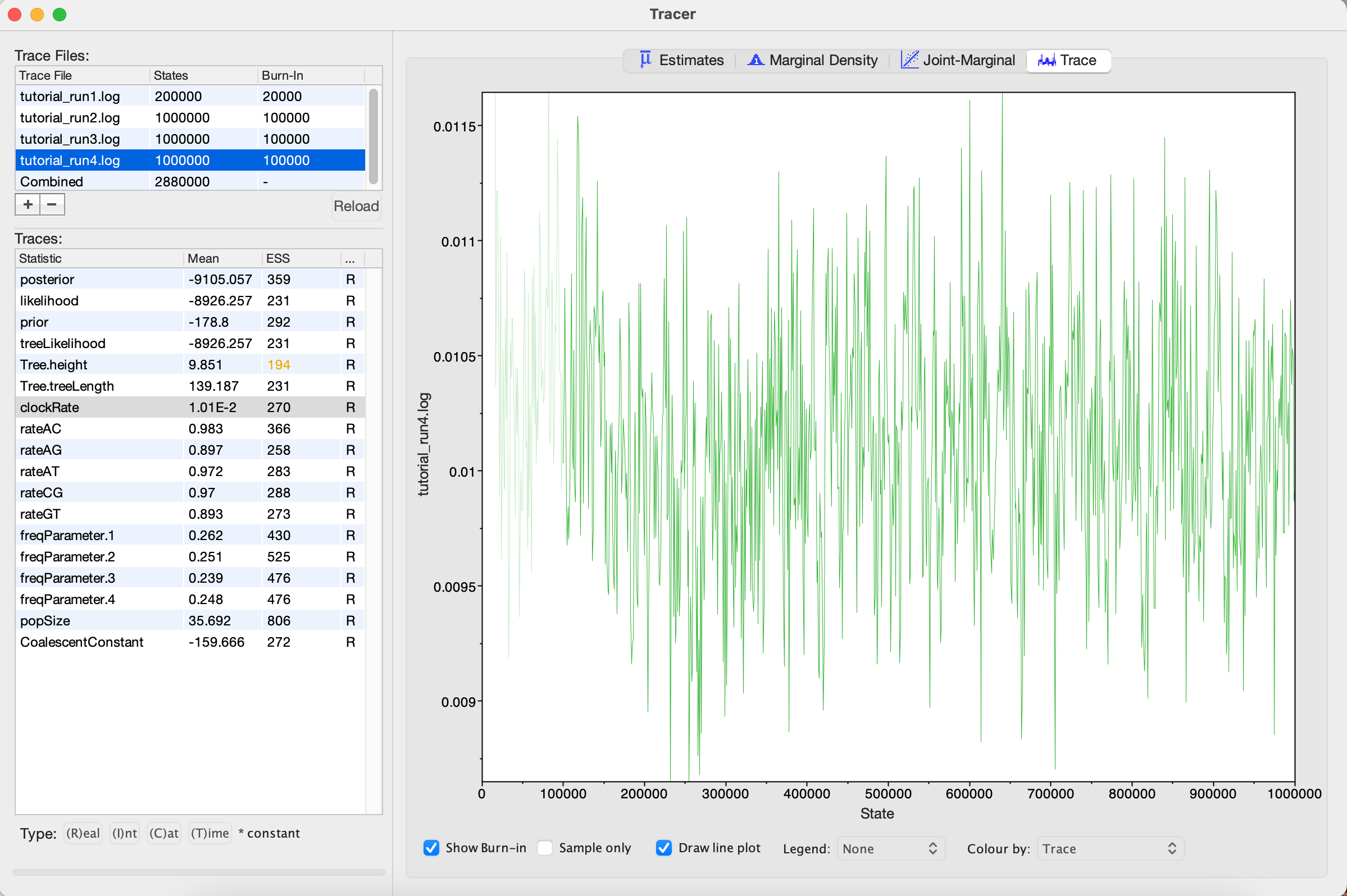
Looking at the MCMC output in Tracer, we see that all parameters are starting to mix well with relatively high ESS values. Personally, I would probably want to run one final MCMC for several million iterations just to be on the safe side, but this can easily be done by adding more iterations to the chain as we did for Run 2. Alternatively, multiple different MCMC runs can be combined using the program LogCombiner that comes packaged with BEAST. This may be better than running one single long analysis, as it allows us to be sure independent runs are converging on similar parameters.
Figure 18: Trace plot of the clock rate parameter- The number of MCMC iterations needed to achieve a reasonable posterior sample in this tutorial was quite small. With larger alignments, much longer chains may be needed.
- In this tutorial we only considered MCMC performance with respect to exploring parameter space, but we also need to consider tree space. One simple diagnostic for checking convergence and mixing in tree space is to look at the trace plot for the tree likelihood. Poor mixing in the tree likelihood can indicate problems exploring tree space.
- It is always a good idea to check your posterior estimates against sampling from the prior.
- Bayesian Evolutionary Analysis with BEAST 2; chapter 10. {% cite BEAST2book2014 --file Troubleshooting/master-refs %}
{% bibliography --cited --file Troubleshooting/master-refs %}

