A MATLAB GUI used for the analysis of soft x-ray angle-resolved photoemission spectroscopy (SX-ARPES) experiments that give direct access to the electronic band-structure of a material. Designed to be directly compatible with the data format of SX-ARPES experiments at the ADRESS beamline, at the Swiss Light Source (SLS) in the Paul Scherrer Institute (PSI), but can be generalised to other data formats if required.
- Download the ARPESGUI repository.
- Open MATLAB and use Set Path in the Home tab to add the ARPESGUI repository and all its sub-folders into its saved search paths.
- Make sure you also use Set Path to add the repository / folder that contains all of the ARPES data to be loaded in to ARPESGUI.
- Type ARPESGUI in the MATLAB command prompt to boot up the GUI.
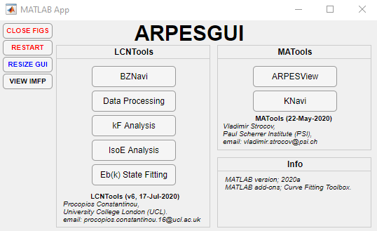
ARPESGUI:
The main menu for all ARPES analysis software in MATLAB, which allows the navigation to and from any piece of analysis UI.
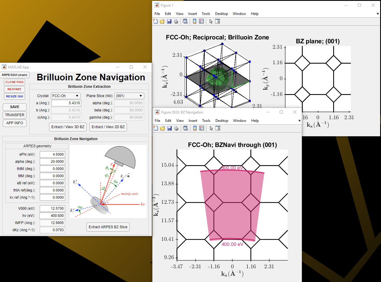
Brilluoin Zone Navigation:
Allows the user to define any crystal geometry and to determine the Wigner-Seitz cell in real-space and the First Brilluoin-Zone in reciprocal space. Additionally, by defining the crystal planes (100), (010) or (001), planar cuts through the stacked Brillouin-Zone can be determined, which is important in the interpretation of ARPES spectra. By imposing the ARPES geometry and experimental variables, the user can define the photon energy being used and extract the ARPES cut/slice being probed through the 2D Brillouin-Zone. This is very useful when it comes to finding what photon energies are needed to probe certain high-symmetry lines or valleys.
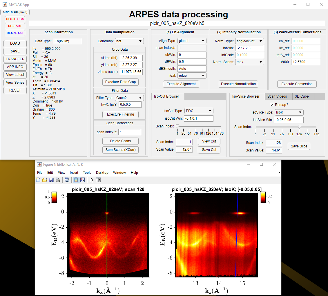
ARPES Data Processing:
Allows the user to walk through all of the processing steps that are required for analysing ARPES spectra, along with several miscellaneous tools that can crop, filter or correct the variables and data associated with the ARPES spectra. The 1st stage is to align the binding energies to the valence band maximum (or Fermi-edge), the 2nd is to normalise the intensity of the ARPES spectra over the scan parameter and the 3rd and final step is to convert the angles into wave-vectors.
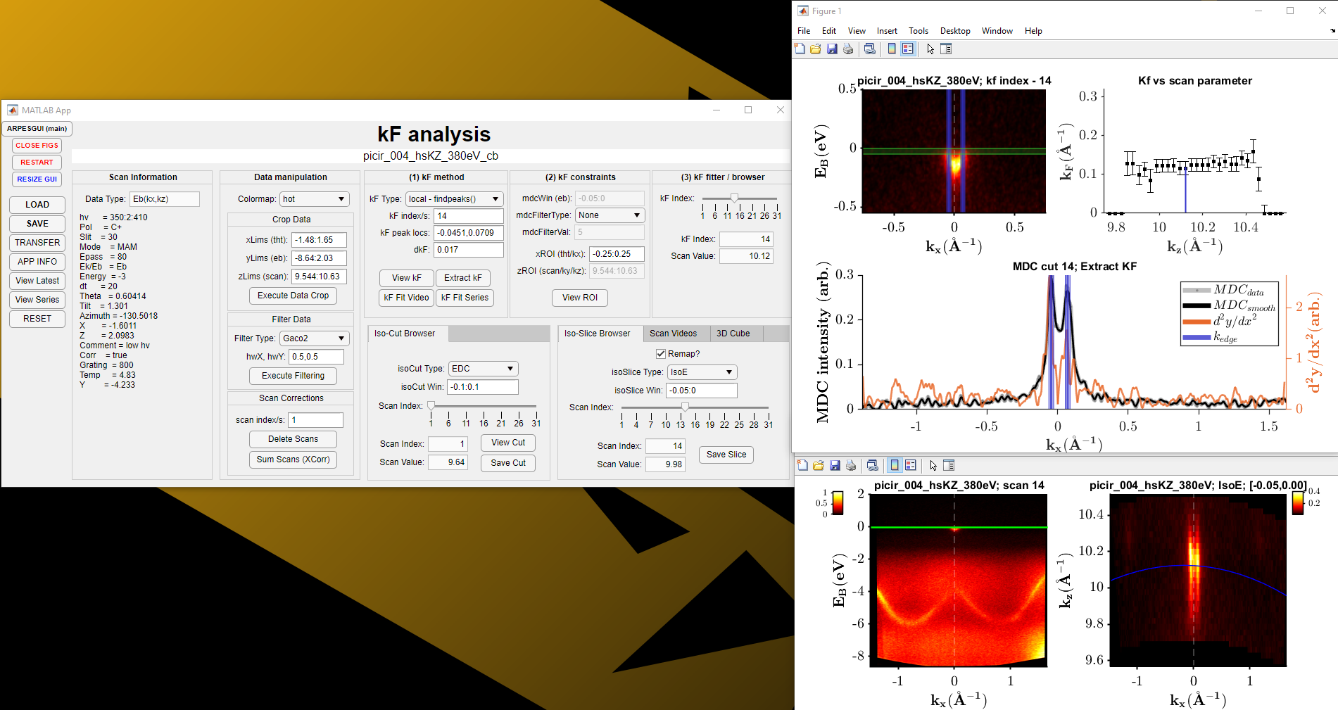
ARPES Kf Analysis:
Allows the user to determine how Kf varies as a function of either the photon energy or tilt angle. This is important when it comes to finding out whether a state is behaving with 2D or 3D characteristics. Can also be used to track how the width of a feature changes as a function of a scan parameter.
IsoE Analysis:
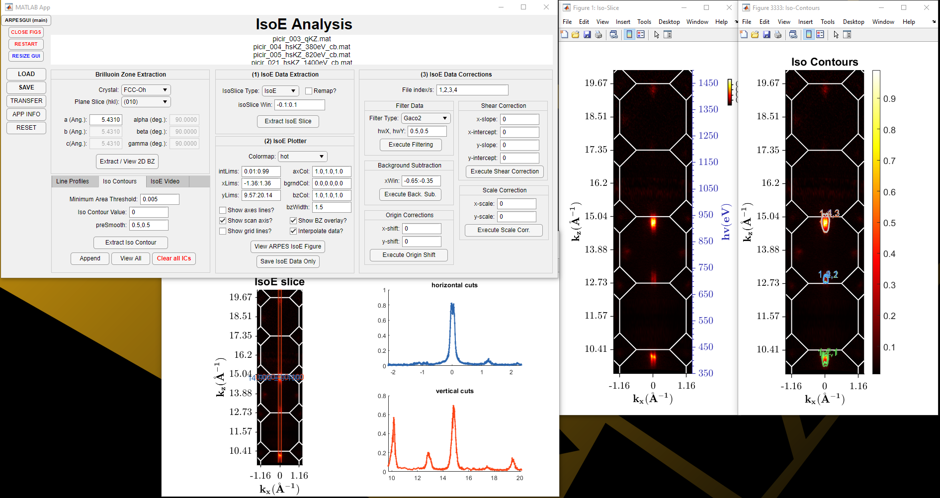
Allows the user to load in single or multiple processed ARPES data-files so that a consistent iso-energetic map can be created even across multiple data-files (if scans were segmented, rather than a single whole scan). The 2D Brillouin-Zone slice can be defined and overlaid on top of the iso-energetic slice. Multiple corrections can also be performed; filtering, background subtraction, origin, shear and scale corrections. There is also the option to determine the area over some threshold, so that the Luttinger Area can be determined to estimate the number density of electrons that are occupying the states.
Eb(k) State Fitting:
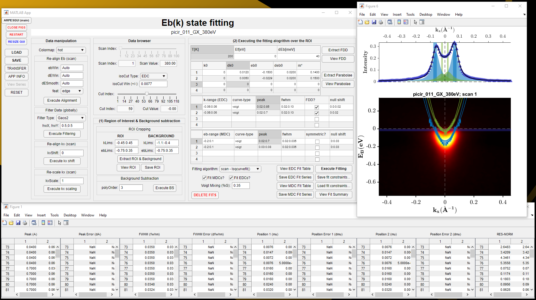
Allows the user to walk through all of the fitting steps to parabolic features within ARPES spectra. The 1st stage is to load in the ARPES data, and perform any pre-fitting corrections (energy re-alignment, resampling, filtering and cropping). The 2nd stage is to crop around the region of interest and also some reference background with the same density of points. The option for polynomial background subtraction is also available using the reference background. The 3rd stage is to the perform the fitting to the parabolic feature using several different approaches and routines. The Fermi-Dirac distribution can be defined and used within the fitting constraints. A parabolic approximation can be set, whose parabolic trail can be used as a constraint to the fitting parameters to allow the solution to converge easier. Various constraints can also be placed on EDC and MDC cuts through the region of interest, but through trial-and-error, the best solution can be found.
MATLAB version: 2020a
MATLAB add-ons: Curve Fitting Toolbox
ARPESGUI & LCNTools:
Procopios Constantinou,
London Centre for Nanotechnology (LCN),
University College London (UCL).
email: procopios.constantinou.16@ucl.ac.uk
MATools functions:
Vladimir Strocov,
Swiss Light Source (SLS),
Paul Scherrer Institute (PSI),
email: vladimir.strocov@psi.ch
This project is licensed under the GNU General Public License v3.0 - see the LICENSE.md file for details.
--PCC July 2020