Adam Lang
Clinical Trial Simulation allows a user to estimate the statistical power of a pre-defined treatment effect at a set of sample sizes. This may be useful in informing recruitment of future clinical trials. Using a Linear-Mixed-Effects Model (LME) trained on pilot data, a user can estimate the power of a treatment effect at a sample size via Monte Carlo Simulation.
Both SampleSizeHelpers.R and SampleSizeEstimationFunction.R must be downloaded. The following packages must be installed:
install.packages("plyr")
install.packages("dplyr")
install.packages("lme4")
install.packages("nlme")
install.packages("simr")
install.packages("stringr")
install.packages("matrixStats")
install.packages("lmerTest")
install.packages("MASS")
install.packages("splitstackshape")
install.packages("cramer")
SampleSizeEstimation requires the following arguments:
-
model A fitted LME model (must be a lmer of package lme4). This model is assumed to have a subject specific random intercept or a subject specific random intercept and slope specified with parentheses.
Ex: “(1|Subject)” “(1+Time|Subject)” -
parameter The name of the rate of change parameter of interest.
Ex: “time”, “t”, “Months” -
pct.change The percent change in the parameter of interest
Ex: .5 (50% improvement) (Either pct.change or delta must be specified, but not both, defaults to NULL) -
delta The change in the pilot estimate of the parameter of interest.
(Either pct.change or delta must be specified, but not both, defaults to NULL) -
time Numeric vector of timepoints.
Ex: c(0, .5, 1, 1.5, 2) -
data Pilot data used to fit pilot model
-
sample_sizes A numeric vector of sample sizes per arm to calculate power.
Ex: c(100, 150, 200, 250) -
nsim Number of iterations to run at each sample size
(defaults to 500) -
sig.level Type I Error rate
defaults to 0.05 -
verbose Print model fit progress
defaults to TRUE -
balance.covariates Character vector of additional covariates to balance while running simulation
defaults to NULL -
test.distribution Compares the distribution of the pilot data to simulated covariates at each bootstrap iteration to ensure similarity. Setting to
TRUEmay increase computation time significantly.defaults to FALSE
SampleSizeEstimation returns a list with the following objects:
Power_Per_Sample data.frame a data.frame with the
power and CI’s at each sample size specified
Run_Time difftime time duration of model fittting
pval.df data.frame a data.frame with dimension nsim
X sample_sizes of p values corresponding to specified treatment
effect.
#Example Data
library(simstudy)

set.seed(123) #for reproducibility

#Creating simulated covariates
def <- defData(     varname = "Int",  dist = "normal",      formula = 25 ,  variance = 7.5, id = "id")
def <- defData(def, varname = "Num1", dist = "normal",      formula = 8  ,  variance = 2, id = "id")
def <- defData(def, varname = "Num2", dist = "normal",      formula = 4   , variance = 1, id = "id")
def <- defData(def, varname = "Cat1", dist = "categorical", formula = ".25 ;.25;.5",      id = "id")
def <- defData(def, varname = "Cat2", dist = "categorical", formula = ".5;.5",            id = "id")
def <- genData(500, def)

#Adding random effects
def <- addCorData(def, idname   = "id", mu  = c(0, 0), sigma   = c(10, 1), rho = .5, corstr = "cs", cnames = c("a0", "a1"))
def <- addPeriods(def, nPeriods = 5, idvars = "id", timevarName = "Time")
def$timeID <- NULL

#Create simulated outcome based on covariates
def2 <- defDataAdd(varname  = "Outcome",
                   formula  = "(Int + a0) + 5*Num1 + 3.5*Num2 + .5*Cat1 - 5*Cat2 + (-2.5 + a1)*period",
                   variance = 10)
def  <- addColumns(def2, def)


def           <- def[,c("id", "period", "Outcome", "Num1", "Num2", "Cat1", "Cat2")]
colnames(def) <- c("Subject", "Time", "Outcome", "Num1", "Num2", "Cat1", "Cat2")
def$Subject   <- factor(def$Subject)
def$Cat1      <- factor(def$Cat1)
def$Cat2      <- factor(def$Cat2)
def <- as.data.frame(def)#fit model
library(lme4)
library(lmerTest)
library(nlme)
library(ggplot2)
simulated.model <- lme4::lmer(Outcome ~ Time + Num1 + Num2 + Cat1 + Cat2 + (1 + Time|Subject), def)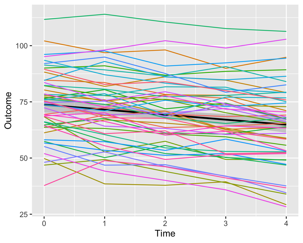
Population model (black) vs subject specific curves
Fixed Effects
##               Estimate Std. Error       df     t value      Pr(>|t|)
## (Intercept) 22.5984099 3.43375705 495.3410   6.5812489  1.190092e-10
## Time        -2.4840735 0.06267994 498.9967 -39.6310751 2.978914e-156
## Num1         4.8168181 0.33663157 493.9729  14.3088722  4.203944e-39
## Num2         3.4474025 0.48413949 493.9726   7.1206803  3.812191e-12
## Cat12        0.5841370 1.32697022 493.9725   0.4402036  6.599822e-01
## Cat13       -0.2204504 1.18164873 493.9725  -0.1865617  8.520809e-01
## Cat22       -4.8025258 0.96057223 493.9725  -4.9996508  7.990883e-07
Random Effects
##  Groups   Name        Std.Dev. Corr
##  Subject  (Intercept) 10.8248
##           Time         1.0106  0.542
##  Residual              3.0709
set.seed(123)
ss.out <- SampleSizeEstimation(model             = simulated.model,
                               parameter         = "Time",
                               pct.change        = 0.3,
                               time              = c(0, 1, 2, 3, 4),
                               data              = def,
                               nsim              = 500,
                               sample_sizes      = c(20, 60, 100),
                               verbose           = FALSE,
test.distribution = FALSE)ss.out$Power_Per_Sample## mean ci.low ci.high SampleSize
## 1 0.382 0.3392193 0.4261847 20
## 2 0.826 0.7898692 0.8582200 60
## 3 0.968 0.9485532 0.9816008 100
Assessing Type I Error is important in bayesian inference as it may not
be controlled at 5%. In order to estimate Type I error rates, a user can
run the simulation with pct.change or delta
set at 0
set.seed(123)
ss.out <- SampleSizeEstimation(model             = simulated.model,
                               parameter         = "Time",
                               pct.change        = 0,
                               time              = c(0, 1, 2, 3, 4),
                               data              = def,
                               nsim              = 500,
                               sample_sizes      = c(20, 60, 100),
                               verbose           = FALSE,
test.distribution = FALSE)ss.out$Power_Per_Sample## mean ci.low ci.high SampleSize
## 1 0.052 0.03424570 0.07526637 20
## 2 0.036 0.02147286 0.05630018 60
## 3 0.050 0.03261518 0.07292762 100
In order to construct the simulated covariate population during the simulation process, a multivariate normal distribution is estimated from the pilot data using the Continuous Method [1]. This requires that all covariate values be positive.
[1] Tannenbaum, Stacey J et al. “Simulation of Correlated Continuous and Categorical Variables Using a Single Multivariate Distribution.” Journal of pharmacokinetics and pharmacodynamics 33.6 (2006): 773–794. Web.
[1] Hadley Wickham (2011). The Split-Apply-Combine Strategy for Data Analysis. Journal of Statistical Software, 40(1), 1-29. URL http://www.jstatsoft.org/v40/i01/.
[2] Hadley Wickham, Romain François, Lionel Henry and Kirill Müller (2021). dplyr: A Grammar of Data Manipulation. R package version 1.0.7. https://CRAN.R-project.org/package=dplyr
[3] Venables, W. N. & Ripley, B. D. (2002) Modern Applied Statistics with S. Fourth Edition. Springer, New York. ISBN 0-387-95457-0
[4] Douglas Bates, Martin Maechler, Ben Bolker, Steve Walker (2015). Fitting Linear Mixed-Effects Models Using lme4. Journal of Statistical Software, 67(1), 1-48. doi:10.18637/jss.v067.i01.
[5] Pinheiro J, Bates D, DebRoy S, Sarkar D, R Core Team (2021). nlme: Linear and Nonlinear Mixed Effects Models. R package version 3.1-153, <URL: https://CRAN.R-project.org/package=nlme>.
[6] Green P, MacLeod CJ (2016). “simr: an R package for power analysis of generalised linear mixed models by simulation.” Methods in Ecology and Evolution, 7(4), 493-498. doi: 10.1111/2041-210X.12504 (URL: https://doi.org/10.1111/2041-210X.12504), <URL: https://CRAN.R-project.org/package=simr>.
[7] Hadley Wickham (2019). stringr: Simple, Consistent Wrappers for Common String Operations. R package version 1.4.0. https://CRAN.R-project.org/package=stringr
[8] Henrik Bengtsson (2020). matrixStats: Functions that Apply to Rows and Columns of Matrices (and to Vectors). R package version 0.57.0. https://CRAN.R-project.org/package=matrixStats
[9] Kuznetsova A, Brockhoff PB, Christensen RHB (2017). “lmerTest Package: Tests in Linear Mixed Effects Models.” Journal of Statistical Software, 82(13), 1-26. doi: 10.18637/jss.v082.i13 (URL: https://doi.org/10.18637/jss.v082.i13).
[10] Venables, W. N. & Ripley, B. D. (2002) Modern Applied Statistics with S. Fourth Edition. Springer, New York. ISBN 0-387-95457-0
[11] Ananda Mahto (2019). splitstackshape: Stack and Reshape Datasets After Splitting Concatenated Values. R package version 1.4.8. https://CRAN.R-project.org/package=splitstackshape
[12] Carsten Franz (2019). cramer: Multivariate Nonparametric Cramer-Test for the Two-Sample-Problem. R package version 0.9-3. https://CRAN.R-project.org/package=cramer
[13] Tannenbaum, Stacey J et al. “Simulation of Correlated Continuous and Categorical Variables Using a Single Multivariate Distribution.” Journal of pharmacokinetics and pharmacodynamics 33.6 (2006): 773–794. Web.