exactplot

The goal of exactplot is to produce millimeter-exact figure layouts and annotate your plots with the full power of Latex. exactplot wraps around tikzDevice and provides utility functions to compose grid plots (e.g., ggplot2 output, but not base plots).

Disclaimer

This is a work-in-progress package and mainly serves as a collection of scripts that I have used in my past papers to produce my scientific figures. I currently do not plan to release it on CRAN and I am only planning to add features if I need them for my work. If you would like to see some feature included, please open a pull request, or feel free to fork the package.

Installation

You can install the development version of exactplot from Github:

devtools::install_github("const-ae/exactplot")

You might need to install additional fonts. By default, exactplot uses the IBM Plex font family. On Mac, you can install them using brew.

brew install --cask font-ibm-plex-sans font-ibm-plex-mono font-ibm-plex-math

Example

library(exactplot)
library(tidyverse)
library(palmerpenguins)

The xp_init function sets consistent fonts and font sizes, adds additional packages to the options("tikzLatexPackages"), and sets the default ggplot2 theme. The default font sizes are available through the xp object. This is needed when you, want to use larger or smaller text in geom_text() (remember to change the size.unit = "pt").

xp_init()
xp$fontsize
#> [1] 8

Make some simple example plots.

scatter_plot <- penguins |>
  mutate(label = paste0(species, " (", island, ", $", year,"$)")) |>
  ggplot(aes(x = flipper_length_mm, y = bill_length_mm)) +
    geom_point(aes(color = species), show.legend = FALSE) +
    geom_label(data = \(x) slice_max(x, bill_length_mm, by = species), 
               aes(label = label, hjust = ifelse(flipper_length_mm < 200, 0, 1)), vjust = -0.2) +
    labs(x = "Flipper length in $10^{-3}$ m", y = "Bill length in $10^{-3}$ m") +
    coord_cartesian(clip = "off")

beak_lengths <- penguins |>
  ggplot(aes(x = bill_length_mm)) +
   geom_density(aes(fill = species), alpha = 0.7 ) +
   labs(x = "Bill length in $10^{-3}$ m")

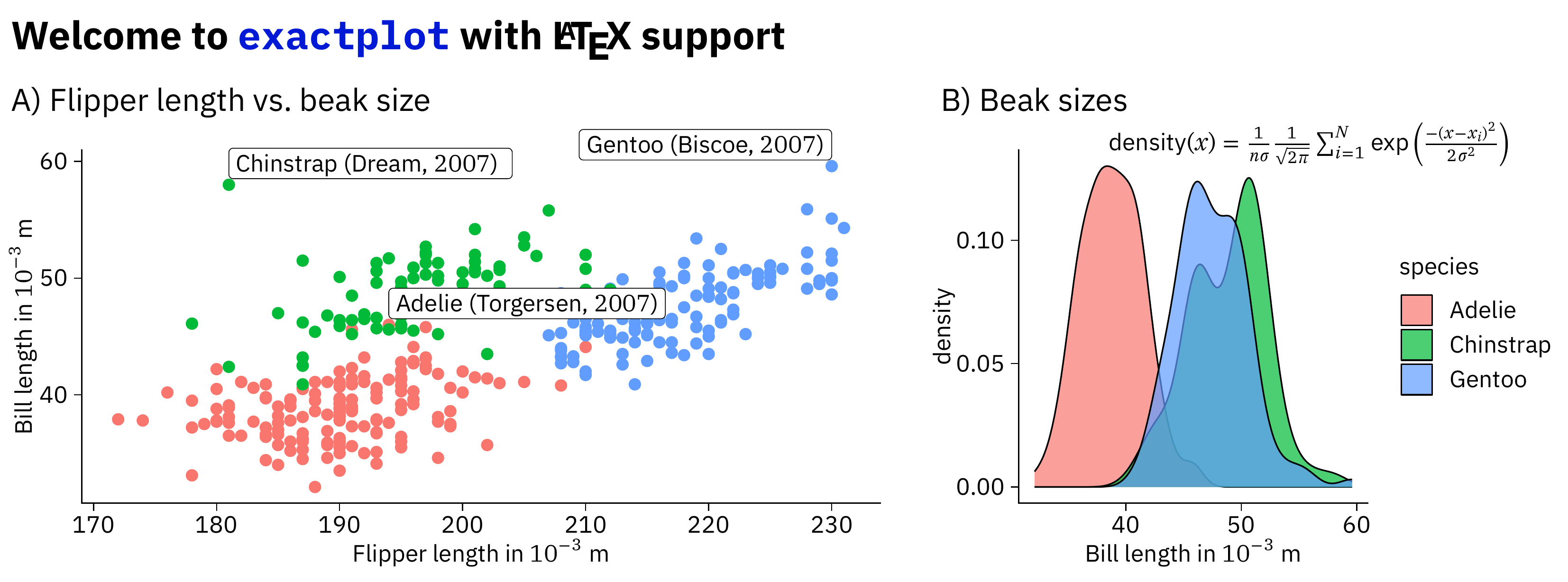
Combine the two plots with some additional annotations. If you call this function without specifying the filename, you get a quick preview without the latex rendering. By default, exactplot uses LuaLatex for rendering, because of its superior font support.

xp_compose_plots(
  xp_text("Welcome to \\texttt{exactplot} with \\LaTeX{} support", x = 1, y = 2, 
          fontsize = xp$fontsize_large, fontface = "bold"),
  xp_text("A) Flipper length vs.\\ beak size", x = 1, y = 8),
  xp_plot(scatter_plot, x = 0, y = 12, width = 80, height = 40),
  
  xp_text("B) Beak sizes", x = 84, y = 8),
  xp_plot(beak_lengths, x = 82, y = 12, width = 58, height = 40),
  xp_text("$\\textrm{density}(x) = \\frac{1}{n\\sigma}\\frac{1}{\\sqrt{2\\pi}}\\sum_{i=1}^N{\\exp\\left(\\frac{-(x-x_i)^2}{2\\sigma^2}\\right)}$",
           x = 99, y = 12, fontsize = xp$fontsize_small),
  
  width = 140, height = 52,
  keep_tex_file = FALSE, filename = "man/example.pdf"
)
#> Using TikZ metrics dictionary at:
#>  README-tikzDictionary
#> gg[gg1]
#> gg[gg2]
#> Warning: Removed 2 rows containing missing values or values outside the scale range
#> (`geom_point()`).
#> gg[gg3]
#> gg[gg4]
#> Warning: Removed 2 rows containing non-finite outside the scale range
#> (`stat_density()`).
#> gg[gg5]
#> gg[gg6]
#> [1] "example.pdf"

Display the output:

print(magick::image_read_pdf("man/example.pdf", density = 600), info = FALSE)