The goal of proDA is to identify differentially abundant proteins in
label-free mass spectrometry data. The main challenge of this data are
the many missing values. The missing values don’t occur randomly but
especially at low intensities. This means that they cannot just be
ignored. Existing methods have mostly focused on replacing the missing
values with some reasonable number (“imputation”) and then run classical
methods. But imputation is problematic because it obscures the amount of
available information. Which in turn can lead to over-confident
predictions.
proDA on the other hand does not impute missing values, but constructs
a probabilistic dropout model. For each sample it fits a sigmoidal
dropout curve. This information can then be used to infer means across
samples and the associated uncertainty, without the intermediate
imputation step. proDA supports full linear models with variance and
location moderation.
For full details, please see our preprint:
Constantin Ahlmann-Eltze and Simon Anders: proDA: Probabilistic Dropout Analysis for Identifying Differentially Abundant Proteins in Label-Free Mass Spectrometry. biorXiv 661496 (Jun 2019)
proDA is implemented as an R package.
You can install it from Bioconductor by typing the following commands into R:
if(!requireNamespace("BiocManager", quietly = TRUE))
    install.packages("BiocManager")
BiocManager::install("proDA")
To get the latest development version from
GitHub, you can use the
devtools package:
# install.packages("devtools")
devtools::install_github("const-ae/proDA")
The pkgdown documentation for the package is available on https://const-ae.github.io/proDA/reference.
In the following section, I will give a very brief overview on the main
functionality of the proDA package, aimed at experienced R users. New
users are advised to skip this “quickstart” and to go directly to
section 1.3, where I give a complete walkthrough and explain in detail,
what steps are necessary for the analysis of label-free mass
spectrometry data.
The three steps that are necessary to analyze the data are
- Load the data (see vignette on loading MaxQuant output files)
- Fit the probabilistic dropout model (
proDA()) - Test in which proteins the coefficients of the model differ
(
test_diff())
# Load the package
library(proDA)
# Generate some dataset with known structure
syn_dataset <- generate_synthetic_data(n_proteins = 100, n_conditions = 2)

# The abundance matrix
syn_dataset$Y[1:5, ]
#>           Condition_1-1 Condition_1-2 Condition_1-3 Condition_2-1 Condition_2-2 Condition_2-3
#> protein_1            NA            NA      18.88592            NA      18.72059      20.06119
#> protein_2      21.37123      20.53557      18.83239      20.41027      21.73266      21.16719
#> protein_3            NA      18.77742      18.98681            NA            NA      19.20291
#> protein_4      25.44209      25.15151      25.38142      25.22754      24.95229      24.97185
#> protein_5      23.46724      23.15808      23.21357      23.29562      23.25999      23.57925

# Assignment of the samples to the two conditions
syn_dataset$groups
#> [1] Condition_1 Condition_1 Condition_1 Condition_2 Condition_2 Condition_2
#> Levels: Condition_1 Condition_2

# Fit the probabilistic dropout model
fit <- proDA(syn_dataset$Y, design = syn_dataset$groups)

# Identify which proteins differ between Condition 1 and 2
test_diff(fit, `Condition_1` - `Condition_2`, sort_by = "pval", n_max = 5)
#> # A tibble: 5 x 10
#>   name              pval adj_pval  diff t_statistic    se    df avg_abundance n_approx n_obs
#>   <chr>            <dbl>    <dbl> <dbl>       <dbl> <dbl> <dbl>         <dbl>    <dbl> <dbl>
#> 1 protein_96  0.00000248 0.000248  8.62        39.4 0.219     4          22.2     4.02     4
#> 2 protein_95  0.0000103  0.000513 -4.84       -27.6 0.175     4          21.2     6.       6
#> 3 protein_91  0.0000528  0.00176  -4.17       -18.3 0.228     4          19.1     4.01     4
#> 4 protein_98  0.000236   0.00479   4.35        12.5 0.348     4          21.6     6.00     6
#> 5 protein_100 0.000239   0.00479   2.49        12.5 0.200     4          21.3     4.95     5
Other helpful functions for quality control are median_normalization()
and dist_approx().
proDA is an R package that implements a powerful probabilistic dropout
model to identify differentially abundant proteins. The package was
specifically designed for label-free mass spectrometry data and in
particular how to handle the many many missing values.
But all this is useless if you cannot load your data and get it into a shape that is useable. In the next section, I will explain how to load the abundance matrix and bring it into a useful form. The steps that I will go through are
- Load the
proteinGroups.txtMaxQuant output table - Extract the intensity columns and create the abundance matrix
- Replace the zeros with
NAs and take thelog2()of the data - Normalize the data using
median_normalization() - Inspect sample structure with a heatmap of the distance matrix
(
dist_approx()) - Fit the probabilistic dropout model with
proDA() - Identify differentially abundant proteins with
test_diff()
I will now demonstrate how to load a MaxQuant output file. For more information about other approaches for loading the data, please take a look at the vignette on loading data.
MaxQuant is one of the most popular tools for handling raw MS data. It
produces a number of files. The important file that contains the protein
intensities is called proteinGroups.txt. It is a large table with
detailed information about the identification and quantification process
for each protein group (which I will from now on just call “protein”).
This package comes with an example proteinGroups.txt file, located in
the package folder. The file contains the reduced output from an
experiment studying the different DHHCs in Drosophila
melanogaster.
system.file("extdata/proteinGroups.txt", package = "proDA", mustWork = TRUE)
#> [1] "/Users/ahlmanne/Library/R/3.6/library/proDA/extdata/proteinGroups.txt"
In this example, I will use the base R functions to load the data, because they don’t require any additional dependencies.
# Load the table into memory
maxquant_protein_table <- read.delim(
    system.file("extdata/proteinGroups.txt", package = "proDA", mustWork = TRUE),
    stringsAsFactors = FALSE
)
As I have mentioned, the table contains a lot of information (359 columns!!), but we are first of all interested in the columns which contain the measured intensities.
# I use a regular expression (regex) to select the intensity columns
intensity_colnames <- grep("^LFQ\\.intensity\\.", colnames(maxquant_protein_table), value=TRUE)
head(intensity_colnames)
#> [1] "LFQ.intensity.CG1407.01" "LFQ.intensity.CG1407.02" "LFQ.intensity.CG1407.03"
#> [4] "LFQ.intensity.CG4676.01" "LFQ.intensity.CG4676.02" "LFQ.intensity.CG4676.03"


# Create the intensity matrix
abundance_matrix <- as.matrix(maxquant_protein_table[, intensity_colnames])
# Adapt column and row maxquant_protein_table
colnames(abundance_matrix) <- sub("^LFQ\\.intensity\\.", "", intensity_colnames)
rownames(abundance_matrix) <- maxquant_protein_table$Protein.IDs
# Print some rows of the matrix with short names so they fit on the screen
abundance_matrix[46:48, 1:6]
#>                                       CG1407.01 CG1407.02 CG1407.03 CG4676.01 CG4676.02 CG4676.03
#> A0A0B4K6W1;P08970                        713400    845440         0         0   1032600         0
#> A0A0B4K6W2;A0A0B4K7S0;P55824-3;P55824   5018800   4429500   2667200         0   8780200   1395800
#> A0A0B4K6X7;A1Z8J0                             0         0         0         0         0         0
After extracting the bits from the table we most care about, we will have to modify it.
Firstly, MaxQuant codes missing values as 0. This is misleading,
because the actual abundance probably was not zero, but just some value
too small to be detected by the mass spectrometer. Accordingly, I will
replace all 0 with NA.
Secondly, the raw intensity values have a linear mean-variance relation.
This is undesirable, because a change of x units can be a large shift
if the mean is small or irrelevant if the mean is large. Luckily, to
make the mean and variance independent, we can just log the
intensities. Now a change of x units is as significant for highly
abundant proteins, as it is for low abundant ones.
abundance_matrix[abundance_matrix == 0] <- NA
abundance_matrix <- log2(abundance_matrix)
abundance_matrix[46:48, 1:6]
#>                                       CG1407.01 CG1407.02 CG1407.03 CG4676.01 CG4676.02 CG4676.03
#> A0A0B4K6W1;P08970                      19.44435  19.68934        NA        NA  19.97785        NA
#> A0A0B4K6W2;A0A0B4K7S0;P55824-3;P55824  22.25891  22.07871  21.34689        NA  23.06582  20.41266
#> A0A0B4K6X7;A1Z8J0                            NA        NA        NA        NA        NA        NA
Quality control (QC) is essential for a successful bioinformatics analysis, because any dataset shows some unwanted variation or could even contain more serious error like for example a sample swap.
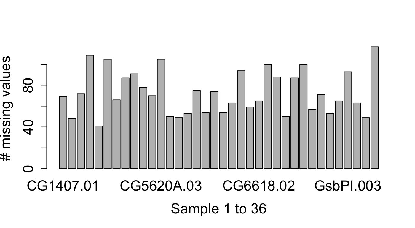
Often we start with normalizing the data to remove potential sample specific effects. But already this step is challenging, because the missing values cannot easily be corrected for. Thus, a first helpful plot is to look how many missing values are in each sample.
barplot(colSums(is.na(abundance_matrix)),
        ylab = "# missing values",
        xlab = "Sample 1 to 36")
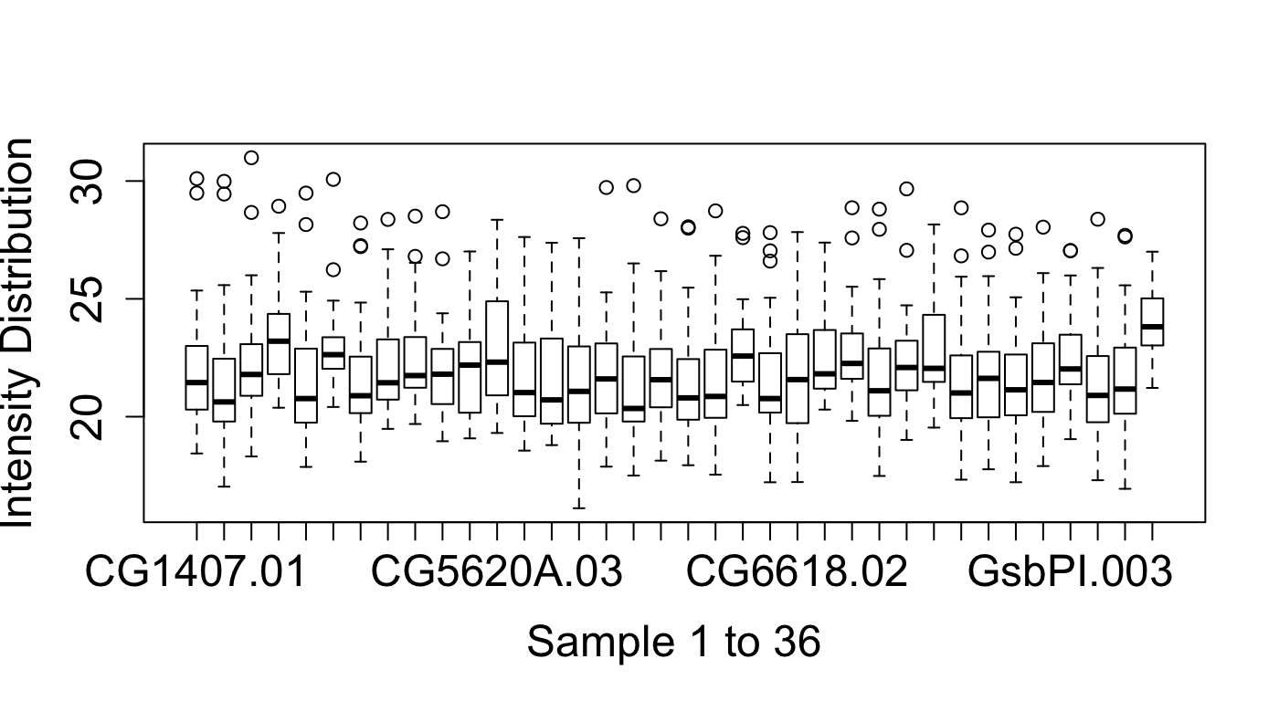
We can see that the number of missing values differs substantially between samples (between 30% and 90%) in this dataset. If we take a look at the intensity distribution for each sample, we see that they differ substantially as well.
boxplot(abundance_matrix,
        ylab = "Intensity Distribution",
        xlab = "Sample 1 to 36")
Note that, the intensity distribution is shifted upwards for samples which also have a large number of missing values (for example the last one). This agrees with our idea that small values are more likely to be missing. On the other hand, this also demonstrates why normalization methods such as quantile normalization, which distort the data until all the distributions are equal, are problematic. I will apply the more “conservative” median normalization, which ignores the missing values and transforms the values so that the median difference between the sample and average across all other samples is zero.
normalized_abundance_matrix <- median_normalization(abundance_matrix)An important tool to identify sample swaps and outliers in the dataset is to look at the sample distance matrix. It shows the distances of samples A to B, A to C, B to C and so on.
The base R dist() function can not handle input data that contains
missing values, so we might be tempted to just replace the missing
values with some realistic numbers and calculate the distance on the
completed dataset. But choosing a good replacement value is challenging
and can also be misleading because the samples with many missing values
would be considered too close.
Instead proDA provides the dist_approx() function that takes either
a fitted model (ie. the output from proDA()) or a simple matrix (for
which it internally calls proDA()) and estimates the expected distance
without imputing the missing values. In addition, it reports the
associated uncertainty with every estimate. The estimates for samples
with many missing values will be uncertain, allowing the data analyst to
discount them.
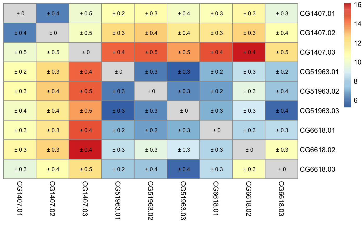
da <- dist_approx(normalized_abundance_matrix)dist_approx() returns two elements the mean of the estimate and the
associated sd. In the next step I will plot the heatmap for three
different conditions, adding the 95% confidence interval as text to each
cell.
# This chunk only works if pheatmap is installed
# install.packages("pheatmap")
sel <- c(1:3,  # CG1407
         7:9,  # CG59163
         22:24)# CG6618

plot_mat <- as.matrix(da$mean)[sel, sel]
# Remove diagonal elements, so that the colorscale is not distorted
plot_mat[diag(9) == 1] <- NA
# 95% conf interval is approx `sd * 1.96`
uncertainty <- matrix(paste0(" ± ",round(as.matrix(da$sd * 1.96)[sel, sel], 1)), nrow=9)
pheatmap::pheatmap(plot_mat,
                   cluster_rows = FALSE, cluster_cols = FALSE,
                   display_numbers= uncertainty,
number_color = "black")In the next step, we will fit the actual linear probabilistic dropout model to the normalized data. But before we start, I will create a data.frame that contains some additional information on each sample, in particular to which condition that sample belongs.
# The best way to create this data.frame depends on the column naming scheme
sample_info_df <- data.frame(name = colnames(normalized_abundance_matrix),
                             stringsAsFactors = FALSE)
sample_info_df$condition <- substr(sample_info_df$name, 1, nchar(sample_info_df$name)  - 3)
sample_info_df$replicate <- as.numeric(
  substr(sample_info_df$name, nchar(sample_info_df$name)  - 1, 20)
)
sample_info_df
#> # A tibble: 36 x 3
#>    name       condition replicate
#>    <chr>      <chr>         <dbl>
#>  1 CG1407.01  CG1407            1
#>  2 CG1407.02  CG1407            2
#>  3 CG1407.03  CG1407            3
#>  4 CG4676.01  CG4676            1
#>  5 CG4676.02  CG4676            2
#>  6 CG4676.03  CG4676            3
#>  7 CG51963.01 CG51963           1
#>  8 CG51963.02 CG51963           2
#>  9 CG51963.03 CG51963           3
#> 10 CG5620A.01 CG5620A           1
#> # … with 26 more rows
Now we can call the proDA() function to actually fit the model. We
specify the design using the formula notation, referencing the
condition column in the sample_info_df data.frame that we have just
created. In addition, I specify that I want to use the S2R condition
as the reference because I know that it was the negative control and
this way automatically all coefficients measure how much each condition
differs from the negative control.
fit <- proDA(normalized_abundance_matrix, design = ~ condition,
             col_data = sample_info_df, reference_level = "S2R")
fit
#>  Parameters of the probabilistic dropout model
#>
#> The dataset contains 36 samples and 122 proteins
#> 59.7% of the values are missing
#>
#> Experimental design: y~condition
#> The model has successfully converged.
#>
#> The inferred parameters are:
#> location_prior_mean:     19.5
#> location_prior_scale:    8.37
#> location_prior_df:       3
#> variance_prior_scale:    0.283
#> variance_prior_df:       1.64
#> dropout_curve_position:  19.9, 19, 20.1, 22.8, ...
#> dropout_curve_scale:     -0.816, -0.601, -1.02, -1.3, ...
The proDAFit object prints a number of useful information about the
convergence of the model, the size of the dataset, the number of missing
values, and the inferred hyper parameters.
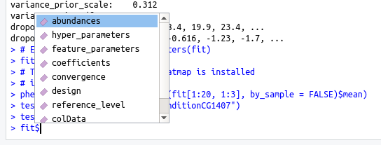
To make it easy to find available methods on the proDAFit object, the
$-operator is overloaded and shows a list of possible functions:
# Equivalent to feature_parameters(fit)
fit$feature_parameters
#> # A tibble: 122 x 4
#>    n_approx     df       s2 n_obs
#>       <dbl>  <dbl>    <dbl> <dbl>
#>  1     12.0  0.001 3808.        5
#>  2     12.0  0.001 2439.        1
#>  3     19.3  8.93     4.07     14
#>  4     12.0  0.001  850.        6
#>  5     17.4  7.04     0.470    17
#>  6     12.0  0.001 2472.        1
#>  7     12.0  0.001 2410.        1
#>  8     28.9 18.6      0.217    29
#>  9     12.0  0.001 1797.        4
#> 10     12.0  0.001 1881.        4
#> # … with 112 more rows
Internally the proDAFit object is implemented as a subclass of
SummarizedExperiment. This means it can be subsetted, which is for
example useful for calculating the distance of a subset of proteins and
samples.
# This chunk only works if pheatmap is installed
# install.packages("pheatmap")
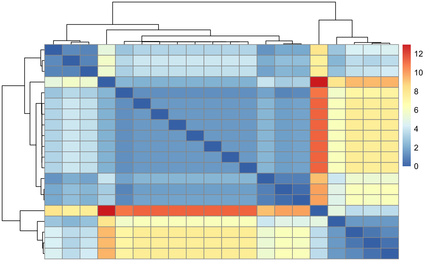
pheatmap::pheatmap(dist_approx(fit[1:20, 1:3], by_sample = FALSE)$mean)Lastly, we will use a Wald test to identify in which proteins a
coefficient is significantly different from zero. The test_diff()
function takes first the fit object produced by proDA() and a contrast
argument. This can either be a string or an expression if we want to
test more complex combinations. For example conditionCG1407 - (conditionCG6017 + conditionCG5880) / 2 would test for the difference
between CG1407 and the average of CG6017 and CG5880.
Alternatively test_diff() also supports likelihood ratio F-tests. In
that case instead of the contrast argument specify the reduced_model
argument.
# Test which proteins differ between condition CG1407 and S2R
# S2R is the default contrast, because it was specified as the `reference_level`
test_res <- test_diff(fit, "conditionCG1407")
test_res
#> # A tibble: 122 x 10
#>    name                   pval adj_pval    diff t_statistic    se    df avg_abundance n_approx n_obs
#>    <chr>                 <dbl>    <dbl>   <dbl>       <dbl> <dbl> <dbl>         <dbl>    <dbl> <dbl>
#>  1 Q8IP47;Q9VJP8;Q9V43… 0.904     0.964 -0.132      -0.122  1.08     24          18.9     12.0     5
#>  2 A0A023GPV6;A8JV04;Q… 0.923     0.964 -0.0993     -0.0979 1.01     24          18.4     12.0     1
#>  3 A0A023GQA5;P24156    0.0356    0.265 -2.92       -2.23   1.31     24          19.3     19.3    14
#>  4 Q1RKY1;A0A0B4LG19;A… 0.667     0.964  0.632       0.435  1.45     24          18.7     12.0     6
#>  5 A0A0B4JD00;A8DY69;I… 0.919     0.964  0.0689      0.103  0.670    24          20.0     17.4    17
#>  6 A0A0B4JCT8;Q9V780    0.923     0.964 -0.0995     -0.0981 1.01     24          18.5     12.0     1
#>  7 A0A0B4LHQ4;A0A0B4JD… 0.923     0.964 -0.0991     -0.0977 1.01     24          18.4     12.0     1
#>  8 A0A0B4JCW4;Q9VHJ8;Q… 0.643     0.964 -0.197      -0.469  0.419    24          21.9     28.9    29
#>  9 Q9VDV4;A0A0B4JCY1;Q… 0.295     0.861  1.95        1.07   1.82     24          18.7     12.0     4
#> 10 A0A0B4JCY6;Q7KSF4;A… 0.598     0.964 -0.783      -0.535  1.46     24          19.0     12.0     4
#> # … with 112 more rows
This walkthrough ends with the identification which proteins are differentially abundant. But for a real dataset, now the actual analysis only just begins. A list of significant proteins is hardly ever a publishable result, one often needs to make sense what the relevant underlying biological mechanisms are. But for this problem other tools are necessary, which depend on the precise question associated with the biological problem at hand.
sessionInfo()
#> R version 3.6.1 (2019-07-05)
#> Platform: x86_64-apple-darwin15.6.0 (64-bit)
#> Running under: macOS Mojave 10.14.6
#>
#> Matrix products: default
#> BLAS:   /Library/Frameworks/R.framework/Versions/3.6/Resources/lib/libRblas.0.dylib
#> LAPACK: /Library/Frameworks/R.framework/Versions/3.6/Resources/lib/libRlapack.dylib
#>
#> locale:
#> [1] en_US.UTF-8/en_US.UTF-8/en_US.UTF-8/C/en_US.UTF-8/en_US.UTF-8
#>
#> attached base packages:
#> [1] stats     graphics  grDevices utils     datasets  methods   base
#>
#> other attached packages:
#> [1] proDA_0.99.7
#>
#> loaded via a namespace (and not attached):
#>  [1] Rcpp_1.0.1                  RColorBrewer_1.1-2          pillar_1.4.2
#>  [4] compiler_3.6.1              GenomeInfoDb_1.20.0         XVector_0.24.0
#>  [7] bitops_1.0-6                tools_3.6.1                 zlibbioc_1.30.0
#> [10] zeallot_0.1.0               digest_0.6.20               gtable_0.3.0
#> [13] evaluate_0.14               tibble_2.1.3                lattice_0.20-38
#> [16] pkgconfig_2.0.2             rlang_0.4.0                 Matrix_1.2-17
#> [19] cli_1.1.0                   DelayedArray_0.10.0         rstudioapi_0.10
#> [22] yaml_2.2.0                  parallel_3.6.1              xfun_0.8
#> [25] GenomeInfoDbData_1.2.1      stringr_1.4.0               extraDistr_1.8.11
#> [28] knitr_1.23                  vctrs_0.2.0                 S4Vectors_0.22.0
#> [31] IRanges_2.18.1              stats4_3.6.1                grid_3.6.1
#> [34] Biobase_2.44.0              fansi_0.4.0                 BiocParallel_1.18.0
#> [37] rmarkdown_1.13              pheatmap_1.0.12             magrittr_1.5
#> [40] scales_1.0.0                backports_1.1.4             htmltools_0.3.6
#> [43] matrixStats_0.54.0          BiocGenerics_0.30.0         GenomicRanges_1.36.0
#> [46] assertthat_0.2.1            SummarizedExperiment_1.14.0 colorspace_1.4-1
#> [49] utf8_1.1.4                  stringi_1.4.3               munsell_0.5.0
#> [52] RCurl_1.95-4.12             crayon_1.3.4