📦 microViz is an R package for analysis and visualization of
microbiome sequencing data.
🔨 microViz functions are intended to be beginner-friendly but
flexible.
🔬 microViz extends or complements popular microbial ecology
packages, including phyloseq, vegan, & microbiome.
📎 This website is the best place for documentation and examples: https://david-barnett.github.io/microViz/
-
This ReadMe shows a few example analyses
-
The Getting Started guide shows more example analyses and gives advice on using microViz with your own data
-
The Reference page lists all functions and links to help pages and examples
-
The News page describes important changes in new microViz package versions
-
The Articles pages give tutorials and further examples
-
Post on GitHub discussions if you have questions/requests
microViz is not (yet) available from CRAN. You can install microViz from R Universe, or from GitHub.
I recommend you first install the Bioconductor dependencies using the code below.
if (!requireNamespace("BiocManager", quietly = TRUE)) install.packages("BiocManager")
BiocManager::install(c("phyloseq", "microbiome", "ComplexHeatmap"), update = FALSE)install.packages(
"microViz",
repos = c(davidbarnett = "https://david-barnett.r-universe.dev", getOption("repos"))
)I also recommend you install the following suggested CRAN packages.
install.packages("ggtext") # for rotated labels on ord_plot()
install.packages("ggraph") # for taxatree_plots()
install.packages("DT") # for tax_fix_interactive()
install.packages("corncob") # for beta binomial models in tax_model()# Installing from GitHub requires the remotes package
install.packages("remotes")
# Windows users will also need to have RTools installed! http://jtleek.com/modules/01_DataScientistToolbox/02_10_rtools/
# To install the latest version:
remotes::install_github("david-barnett/microViz")
# To install a specific "release" version of this package, e.g. an old version
remotes::install_github("david-barnett/microViz@0.12.0") 🍎 macOS users - might need to install
xquartz to make the heatmaps work (to do
this with homebrew, run the following command in your mac’s Terminal:
brew install --cask xquartz
📦 I highly recommend using renv for managing your R package installations across multiple projects.
🐳 For Docker users an image with the main branch installed is available at: https://hub.docker.com/r/barnettdavid/microviz-rocker-verse
📅 microViz is tested to work with R version 4.* on Windows, MacOS, and Ubuntu 20. R version 3.6.* should probably work, but I don’t fully test this.
library(microViz)
#> microViz version 0.12.5 - Copyright (C) 2021-2024 David Barnett
#> ! Website: https://david-barnett.github.io/microViz
#> ✔ Useful?  For citation details, run: `citation("microViz")`
#> ✖ Silence? `suppressPackageStartupMessages(library(microViz))`
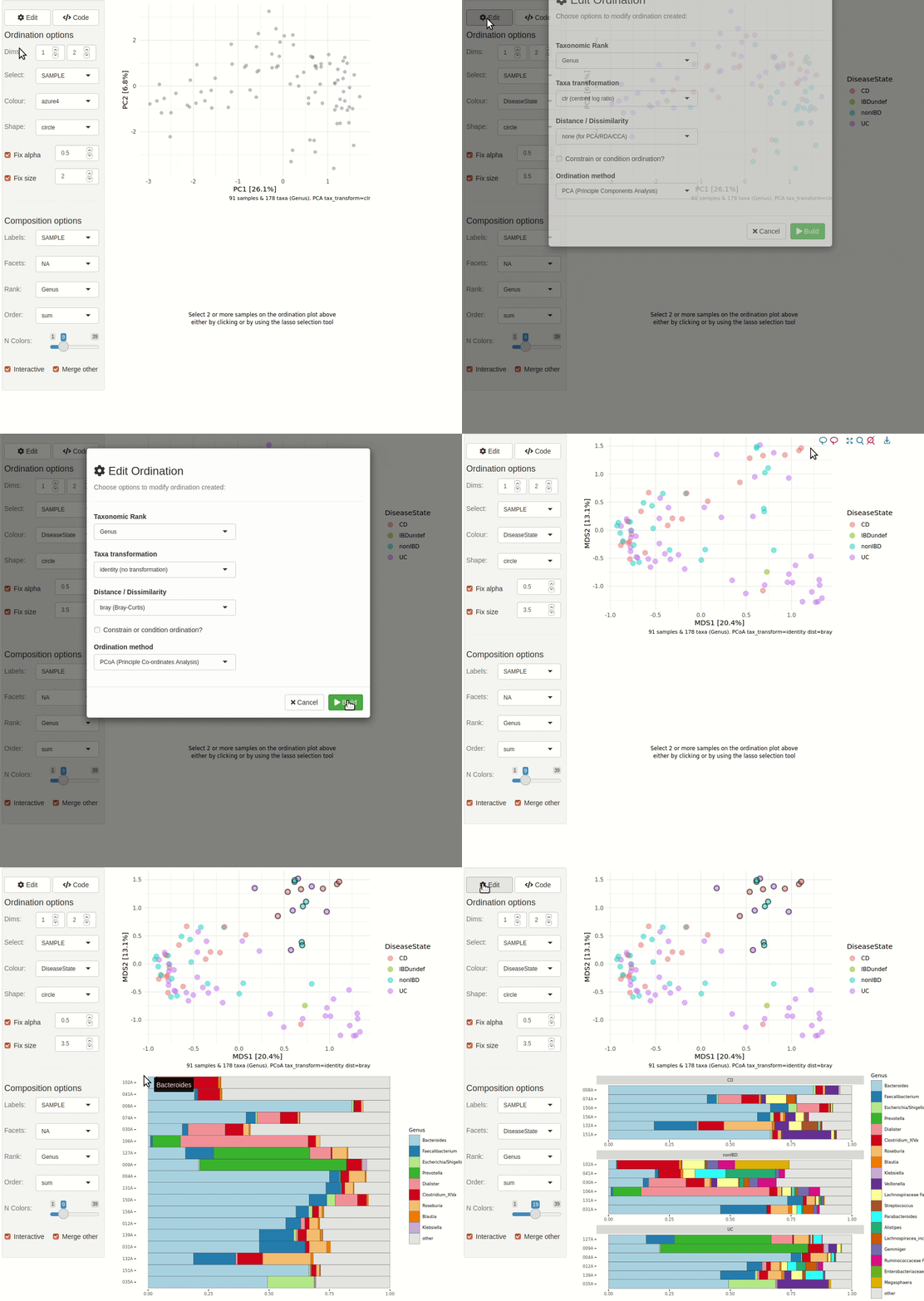
microViz provides a Shiny app for an easy way to start exploring your microbiome data: all you need is a phyloseq object.
# example data from corncob package
pseq <- microViz::ibd %>%
  tax_fix() %>%
phyloseq_validate()ord_explore(pseq) # gif generated with microViz version 0.7.4 (plays at 1.75x speed)library(phyloseq)
library(dplyr)
library(ggplot2)# get some example data
data("dietswap", package = "microbiome")
# create a couple of numerical variables to use as constraints or conditions
dietswap <- dietswap %>%
ps_mutate(
weight = recode(bmi_group, obese = 3, overweight = 2, lean = 1),
female = if_else(sex == "female", true = 1, false = 0),
african = if_else(nationality == "AFR", true = 1, false = 0)
)
# add a couple of missing values to show how microViz handles missing data
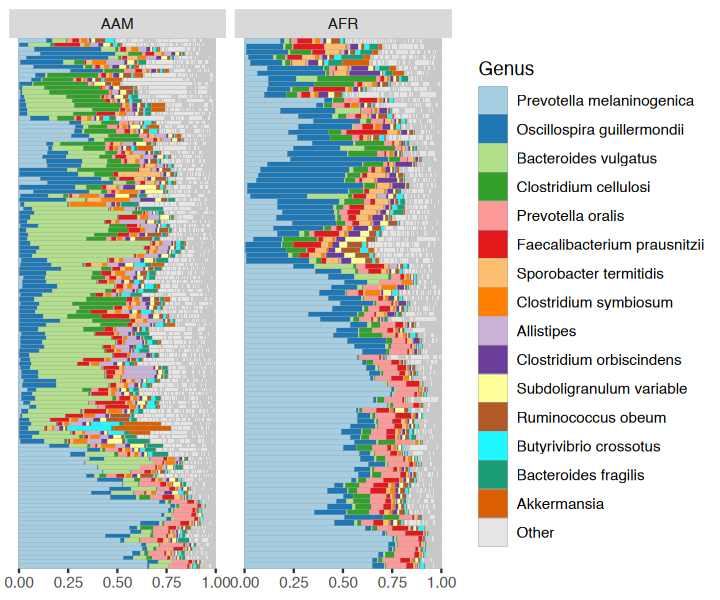
sample_data(dietswap)$african[c(3, 4)] <- NAYou have quite a few samples in your phyloseq object, and would like to visualize their compositions. Perhaps these example data differ by participant nationality?
dietswap %>%
  comp_barplot(
    tax_level = "Genus", n_taxa = 15, other_name = "Other",
    taxon_renamer = function(x) stringr::str_remove(x, " [ae]t rel."),
    palette = distinct_palette(n = 15, add = "grey90"),
    merge_other = FALSE, bar_outline_colour = "darkgrey"
  ) +
  coord_flip() +
  facet_wrap("nationality", nrow = 1, scales = "free") +
  labs(x = NULL, y = NULL) +
  theme(axis.text.y = element_blank(), axis.ticks.y = element_blank())
#> Registered S3 method overwritten by 'seriation':
#>   method         from
#>   reorder.hclust vegan
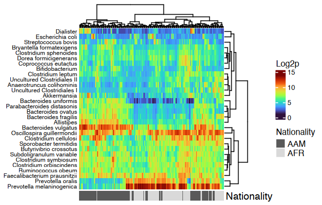
htmp <- dietswap %>%
ps_mutate(nationality = as.character(nationality)) %>%
tax_transform("log2", add = 1, chain = TRUE) %>%
comp_heatmap(
taxa = tax_top(dietswap, n = 30), grid_col = NA, name = "Log2p",
taxon_renamer = function(x) stringr::str_remove(x, " [ae]t rel."),
colors = heat_palette(palette = viridis::turbo(11)),
row_names_side = "left", row_dend_side = "right", sample_side = "bottom",
sample_anno = sampleAnnotation(
Nationality = anno_sample_cat(
var = "nationality", col = c(AAM = "grey35", AFR = "grey85"),
box_col = NA, legend_title = "Nationality", size = grid::unit(4, "mm")
)
)
)
ComplexHeatmap::draw(
object = htmp, annotation_legend_list = attr(htmp, "AnnoLegends"),
merge_legends = TRUE
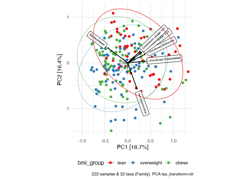
)Ordination methods can also help you to visualize if overall microbial ecosystem composition differs markedly between groups, e.g. BMI.
Here is one option as an example:
- Aggregate the taxa into bacterial families (for example) - use
tax_agg() - Transform the microbial data with the centered-log-ratio
transformation - use
tax_transform() - Perform PCA with the clr-transformed features (equivalent to
Aitchison distance PCoA) - use
ord_calc() - Plot the first 2 axes of this PCA ordination, colouring samples by
group and adding taxon loading arrows to visualize which taxa
generally differ across your samples - use
ord_plot() - Customise the theme of the ggplot as you like and/or add features like ellipses or annotations
# perform ordination
unconstrained_aitchison_pca <- dietswap %>%
  tax_agg("Family") %>%
  tax_transform("clr") %>%
  ord_calc()
# ord_calc will automatically infer you want a "PCA" here
# specify explicitly with method = "PCA", or you can pick another method

# create plot
pca_plot <- unconstrained_aitchison_pca %>%
  ord_plot(
    plot_taxa = 1:6, colour = "bmi_group", size = 1.5,
    tax_vec_length = 0.325,
    tax_lab_style = tax_lab_style(max_angle = 90, aspect_ratio = 1),
    auto_caption = 8
  )

# customise plot
customised_plot <- pca_plot +
  stat_ellipse(aes(linetype = bmi_group, colour = bmi_group), linewidth = 0.3) + # linewidth not size, since ggplot 3.4.0
  scale_colour_brewer(palette = "Set1") +
  theme(legend.position = "bottom") +
  coord_fixed(ratio = 1, clip = "off") # makes rotated labels align correctly

# show plot
customised_plotYou visualised your ordinated data in the plot above. Below you can see how to perform a PERMANOVA to test the significance of BMI’s association with overall microbial composition. This example uses the Family-level Aitchison distance to correspond with the plot above.
# calculate distances
aitchison_dists <- dietswap %>%
  tax_transform("identity", rank = "Family") %>%
  dist_calc("aitchison")

# the more permutations you request, the longer it takes
# but also the more stable and precise your p-values become
aitchison_perm <- aitchison_dists %>%
  dist_permanova(
    seed = 1234, # for set.seed to ensure reproducibility of random process
    n_processes = 1, n_perms = 99, # you should use at least 999!
    variables = "bmi_group"
  )
#> 2024-09-14 21:00:04.03385 - Starting PERMANOVA with 99 perms with 1 processes
#> 2024-09-14 21:00:04.090414 - Finished PERMANOVA

# view the permanova results
perm_get(aitchison_perm) %>% as.data.frame()
#>            Df SumOfSqs         R2        F Pr(>F)
#> bmi_group   2  109.170 0.04104336 4.686602   0.01
#> Residual  219 2550.700 0.95895664       NA     NA
#> Total     221 2659.869 1.00000000       NA     NA

# view the info stored about the distance calculation
info_get(aitchison_perm)
#> psExtra info:
#> tax_agg = "Family" tax_trans = "identity" dist_method = "aitchison"You could visualise the effect of the (numeric/logical) variables in
your permanova directly using the ord_plot function with constraints
(and conditions).
perm2 <- aitchison_dists %>%
  dist_permanova(variables = c("weight", "african", "sex"), seed = 321)
#> Dropping samples with missings: 2
#> 2024-09-14 21:00:04.101656 - Starting PERMANOVA with 999 perms with 1 processes
#> 2024-09-14 21:00:05.739389 - Finished PERMANOVA
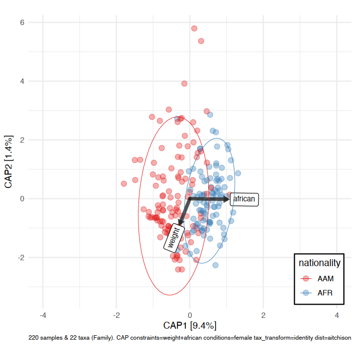
We’ll visualise the effect of nationality and bodyweight on sample composition, after first removing the effect of sex.
perm2 %>%
  ord_calc(constraints = c("weight", "african"), conditions = "female") %>%
  ord_plot(
    colour = "nationality", size = 2.5, alpha = 0.35,
    auto_caption = 7,
    constraint_vec_length = 1,
    constraint_vec_style = vec_constraint(1.5, colour = "grey15"),
    constraint_lab_style = constraint_lab_style(
      max_angle = 90, size = 3, aspect_ratio = 0.8, colour = "black"
    )
  ) +
  stat_ellipse(aes(colour = nationality), linewidth = 0.2) +
  scale_color_brewer(palette = "Set1", guide = guide_legend(position = "inside")) +
  coord_fixed(ratio = 0.8, clip = "off", xlim = c(-4, 4)) +
  theme(legend.position.inside = c(0.9, 0.1), legend.background = element_rect())
#>
#> Centering (mean) and scaling (sd) the constraints and/or conditions:
#>  weight
#>  african
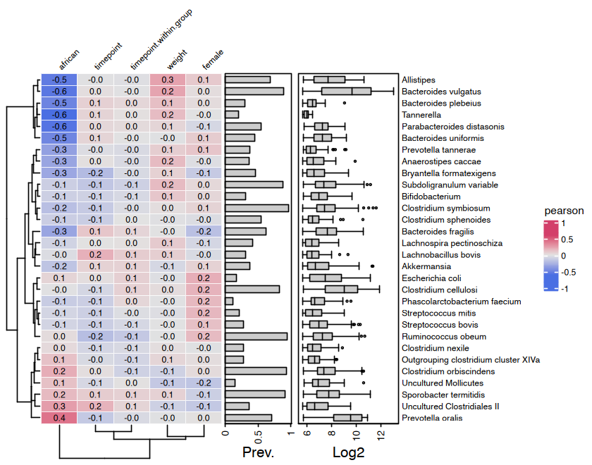
#> femalemicroViz heatmaps are powered by ComplexHeatmap and annotated with
taxa prevalence and/or abundance.
# set up the data with numerical variables and filter to top taxa
psq <- dietswap %>%
  ps_mutate(
    weight = recode(bmi_group, obese = 3, overweight = 2, lean = 1),
    female = if_else(sex == "female", true = 1, false = 0),
    african = if_else(nationality == "AFR", true = 1, false = 0)
  ) %>%
  tax_filter(
    tax_level = "Genus", min_prevalence = 1 / 10, min_sample_abundance = 1 / 10
  ) %>%
  tax_transform("identity", rank = "Genus")
#> Proportional min_prevalence given: 0.1 --> min 23/222 samples.

# randomly select 30 taxa from the 50 most abundant taxa (just for an example)
set.seed(123)
taxa <- sample(tax_top(psq, n = 50), size = 30)
# actually draw the heatmap
cor_heatmap(
  data = psq, taxa = taxa,
  taxon_renamer = function(x) stringr::str_remove(x, " [ae]t rel."),
  tax_anno = taxAnnotation(
    Prev. = anno_tax_prev(undetected = 50),
    Log2 = anno_tax_box(undetected = 50, trans = "log2", zero_replace = 1)
  )
)😇 If you find any part of microViz useful to your work, please consider citing the JOSS article:
Barnett et al., (2021). microViz: an R package for microbiome data visualization and statistics. Journal of Open Source Software, 6(63), 3201, https://doi.org/10.21105/joss.03201
Bug reports, questions, suggestions for new features, and other contributions are all welcome. Feel free to create a GitHub Issue or write on the Discussions page.
This project is released with a Contributor Code of Conduct and by participating in this project you agree to abide by its terms.
sessionInfo()
#> R version 4.4.0 (2024-04-24)
#> Platform: aarch64-apple-darwin20
#> Running under: macOS Sonoma 14.6.1
#>
#> Matrix products: default
#> BLAS:   /Library/Frameworks/R.framework/Versions/4.4-arm64/Resources/lib/libRblas.0.dylib
#> LAPACK: /Library/Frameworks/R.framework/Versions/4.4-arm64/Resources/lib/libRlapack.dylib;  LAPACK version 3.12.0
#>
#> locale:
#> [1] en_US.UTF-8/en_US.UTF-8/en_US.UTF-8/C/en_US.UTF-8/en_US.UTF-8
#>
#> time zone: Europe/Amsterdam
#> tzcode source: internal
#>
#> attached base packages:
#> [1] stats     graphics  grDevices utils     datasets  methods   base
#>
#> other attached packages:
#> [1] ggplot2_3.5.1    dplyr_1.1.4      phyloseq_1.48.0  microViz_0.12.5
#> [5] testthat_3.2.1.1 devtools_2.4.5   usethis_3.0.0
#>
#> loaded via a namespace (and not attached):
#>   [1] RColorBrewer_1.1-3      rstudioapi_0.16.0       jsonlite_1.8.8
#>   [4] shape_1.4.6.1           magrittr_2.0.3          farver_2.1.2
#>   [7] rmarkdown_2.27          GlobalOptions_0.1.2     fs_1.6.4
#>  [10] zlibbioc_1.50.0         vctrs_0.6.5             multtest_2.60.0
#>  [13] memoise_2.0.1           Cairo_1.6-2             htmltools_0.5.8.1
#>  [16] curl_5.2.1              Rhdf5lib_1.26.0         rhdf5_2.48.0
#>  [19] htmlwidgets_1.6.4       plyr_1.8.9              cachem_1.1.0
#>  [22] commonmark_1.9.1        igraph_2.0.3            mime_0.12
#>  [25] lifecycle_1.0.4         iterators_1.0.14        pkgconfig_2.0.3
#>  [28] Matrix_1.7-0            R6_2.5.1                fastmap_1.2.0
#>  [31] clue_0.3-65             GenomeInfoDbData_1.2.12 shiny_1.9.1
#>  [34] digest_0.6.36           selectr_0.4-2           colorspace_2.1-1
#>  [37] S4Vectors_0.42.1        ps_1.7.7                pkgload_1.4.0
#>  [40] seriation_1.5.5         vegan_2.6-6.1           labeling_0.4.3
#>  [43] fansi_1.0.6             httr_1.4.7              mgcv_1.9-1
#>  [46] compiler_4.4.0          remotes_2.5.0           doParallel_1.0.17
#>  [49] withr_3.0.1             viridis_0.6.5           pkgbuild_1.4.4
#>  [52] highr_0.11              MASS_7.3-61             sessioninfo_1.2.2
#>  [55] rjson_0.2.21            biomformat_1.32.0       permute_0.9-7
#>  [58] tools_4.4.0             chromote_0.2.0          ape_5.8
#>  [61] httpuv_1.6.15           glue_1.7.0              nlme_3.1-165
#>  [64] rhdf5filters_1.16.0     promises_1.3.0          gridtext_0.1.5
#>  [67] grid_4.4.0              Rtsne_0.17              cluster_2.1.6
#>  [70] reshape2_1.4.4          ade4_1.7-22             generics_0.1.3
#>  [73] gtable_0.3.5            microbiome_1.26.0       ca_0.71.1
#>  [76] tidyr_1.3.1             websocket_1.4.2         data.table_1.15.4
#>  [79] xml2_1.3.6              utf8_1.2.4              XVector_0.44.0
#>  [82] BiocGenerics_0.50.0     markdown_1.13           foreach_1.5.2
#>  [85] pillar_1.9.0            stringr_1.5.1           later_1.3.2
#>  [88] circlize_0.4.16         splines_4.4.0           ggtext_0.1.2
#>  [91] lattice_0.22-6          survival_3.7-0          tidyselect_1.2.1
#>  [94] registry_0.5-1          ComplexHeatmap_2.20.0   Biostrings_2.72.1
#>  [97] miniUI_0.1.1.1          knitr_1.48              gridExtra_2.3
#> [100] IRanges_2.38.1          stats4_4.4.0            xfun_0.46
#> [103] Biobase_2.64.0          matrixStats_1.3.0       brio_1.1.5
#> [106] stringi_1.8.4           UCSC.utils_1.0.0        yaml_2.3.10
#> [109] evaluate_0.24.0         codetools_0.2-20        tibble_3.2.1
#> [112] cli_3.6.3               xtable_1.8-4            munsell_0.5.1
#> [115] processx_3.8.4          Rcpp_1.0.13             GenomeInfoDb_1.40.1
#> [118] png_0.1-8               parallel_4.4.0          ellipsis_0.3.2
#> [121] profvis_0.3.8           urlchecker_1.0.1        viridisLite_0.4.2
#> [124] scales_1.3.0            purrr_1.0.2             crayon_1.5.3
#> [127] GetoptLong_1.0.5        rlang_1.1.4             TSP_1.2-4
#> [130] rvest_1.0.4