Advanced Lane Finding Project
The goals / steps of this project are the following:
- Compute the camera calibration matrix and distortion coefficients given a set of chessboard images taken by the camera.
- Apply a distortion correction to raw images.
- Use color transforms, gradients, etc., to create a thresholded binary image.
- Apply a perspective transform to rectify binary image ("birds-eye view").
- Detect lane pixels and fit to find the lane boundary.
- Determine the curvature of the lane and vehicle position with respect to center.
- Warp the detected lane boundaries back onto the original image.
- Output visual display of the lane boundaries and numerical estimation of lane curvature and vehicle position.
The code for this step is contained in the cells 2 through 6, of the IPython notebook.
I start by preparing "object points", which will be the (x, y, z) coordinates of the chessboard corners in the world. Here I am assuming the chessboard is fixed on the (x, y) plane at z=0, such that the object points are the same for each calibration image. Thus, objp is just a replicated array of coordinates, and objpoints will be appended with a copy of it every time I successfully detect all chessboard corners in a test image. imgpoints will be appended with the (x, y) pixel position of each of the corners in the image plane with each successful chessboard detection.

I then used the output objpoints and imgpoints to compute the camera calibration and distortion coefficients using the cv2.calibrateCamera() function. I applied this distortion correction to the test image using the cv2.undistort() function and obtained this result:
I used the calibrated camera distortion and transform matrices to perform undistortion and perspective transform of the road images.

The code for my perspective transform includes a function called transform_image(), which appears in cells 7 through 10 of the IPython notebook. The transform_image() function takes as inputs an image (image), as well as camera distortion matrix (camera_matrix) and camera distortion coefficient (camera_distortion). I chose to hardcode the source and destination points in the following manner:
This resulted in the following source and destination points:
| Source | Destination |
|---|---|
| 560, 475 | 270, 275 |
| 726, 475 | 1050, 275 |
| 270, 680 | 270, 680 |
| 1050, 680 | 1050,680 |
I verified that my perspective transform was working as expected by drawing the src and dst points onto a test image and its warped counterpart to verify that the lines appear parallel in the warped image.
I used a combination of HLS color and gradient thresholds to generate a binary image (thresholding steps in 11th cell of notebook). I created a binary image of detected lanes by using the saturation value of the HLS image combined with the detected edges that met the magnitude, direction and absolute threshold values of a Sobel transform. Here's an example of my output for this step.
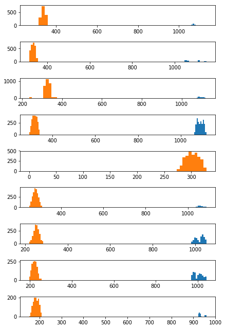
I then proceeded to use the binary image to identify the lane-line pixels by using histograms that summed up the y values along the x axis. I split the image into 9 equal parts horiizontally and created a histogram for each of these parts.
As can be seen in the histograms below, there is a clear cluster of points for each slice representing the left and right lines of the lane. It is worth noting that the right lane in the collection of histograms below only has a large cluster of points in three of them. These three histograms correspond to the three dashed lines visible in the binary image.
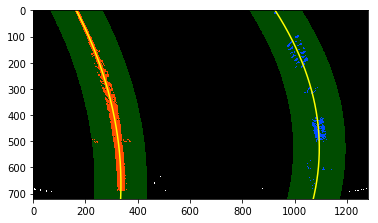
by selecting the x at the maximum y for the lane lines in each histogram, I created a collection of x and y values that were used to mathematically identify the lane. I fit my lane lines with a 2nd order polynomial to get the curve that fits all x an y values for the left and right lines of the lane. The detected curves can be seen in the image below as the yellow lines.
I calculated the radius of curvature for the identified lane lines and the position of the vehicle with respect to the center of the lanes in the 17th cell of notebook.
The radius of curvature was derived by extrapolating the pixel dimensions of the image into real-life measurements based on lane size guidelines by the U.S.D.O.T. In the perspective transformed images, 100px vertically is equal to 3.048 meters, while 700px horizontally is equal to 3.7 meters. I fit my lane lines with a 2nd order polynomial to get the curve that fits all x an y values for the left and right lines using real life dimensions. The resulting curves give us the radius of curvature for each lane line.
The position of the vehicle with respect to the center of the lane was computed by assuming the camera was centered on the vehicle. The difference between the center of the camera image and the detected lane will therefore be the cars position with respect to the center of the lane.
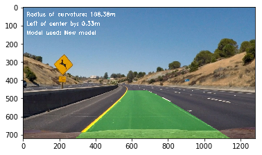
I overlaid the detected lane back unto the perspective transformed image, then performed a reverse transform to get back the original perspective. This can be found on the 18th cell of notebook.
Here's an example of what it looked like after overlaying and performing the reverse transform:
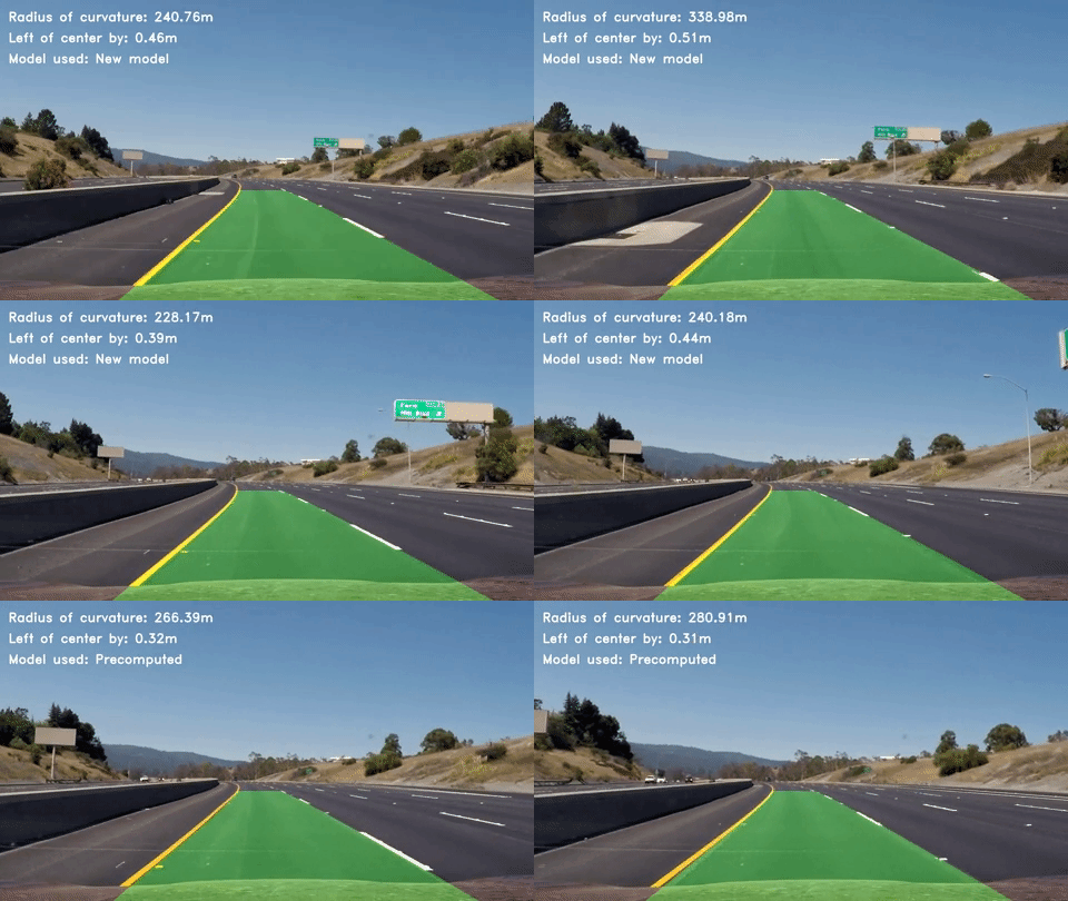
In order to avoid the extensive search and detection of new lanes for every frame of the video, I performed a threshold check to see if the line values of the lane in the new images were similar to previous images. I did this by creating a margin around the previous lane lines to detect what I considered to be similar lane lines.
If a new lane is found to be similar to the previously detected lane, we skip the step of computing a new curve and just use the previous lanes values. In the video, all frames marked New model fell outside our bounds of similarity, while frames marked Precomputed, are based on previously detected lane lines.
The code that checks for similarities and performs calculated estimates can be found in the 13th, 15th and 20th cells of notebook.
Here's a link to my video result
Some potential issues that have not been addressed with my approach is the possibility that intra-lane markings like the HOV/Carpool lane marking might throw off our hsitogram methodology. This will likely throw off lane detection. The same goes for any major transition in material from a black tarred road to a lighter colored concrete road.
Going forward, I could improve this pipeline by performin a sanity check for each detected lane to ensure it doesn't fall outside reasonable bounds of what is expected for the size or curve of a lane. I could also adjust my Saturation and Sobel thresholds further to ensure only the important info is extracted to a binary image.


