Hierarchical probabilistic models for multiple gene/variant associations based on NGS data

The identification of genetic variants affecting gene expression (known as expression quantitative trait loci or eQTLs) is an important step in unravelling the genetic basis of complex traits, including diseases. eQTLseq implements two classes of statistical models for detecting simultaneously multiple associations between gene expression and genomic polymorphisms in a population, using paired DNA-seq and RNA-seq assays as input:

The first class involves Poisson, Binomial and Negative Binomial models, which explicitly model digital gene expression as a function of genetic variation.
The second class involves a Normal/Gaussian model, which relies on appropriate transformations of gene expression data.

All models are embedded in a Bayesian multiple/multivariate regression and variable selection framework. Importantly, in all cases, the posterior probability of multiple gene/variant associations is expressed as a multivariate Normal distribution through the introduction of latent variables, which allows for efficient Bayesian learning. Details of all statistical methods are given in the following paper:

"Hierarchical probabilistic models for multiple gene/variant associations based on NGS data" by Dimitrios V. Vavoulis, Jenny C. Taylor & Anna Schuh, 2017 (submitted)

For further information, please send a message to Dimitris.Vavoulis@ndcls.ox.ac.uk.

Below, you can find instructions for installing and using the software. Enjoy!

Installation

eQTLseq requires Python 3 (I developed it using v3.5). The easiest way to install it is using pip:

me@here:~$ pip install -U eQTLseq

Required dependencies (numpy, scipy, tqdm, rpy2) will be installed automatically. I strongly recommend installing inside a fresh virtual environment. You can create one using something like: python3 -m venv ~/path/to/your/virtual/environments/test.

Usage

Let's see how eQTLseq works on a simulated dataset. Save this in a convenient location and, from an ipython console or notebook, do the following:

## imports data
import pickle as pkl
import numpy as num
import numpy.random as rnd
import matplotlib.pyplot as plt

## load data
with open('/path/to/simdata_1_4_0_0.pkl', 'rb') as fh:
  data = pkl.load(fh)

Z = data['Z']     # simulated expression data
G = data['G']     # simulated genotypes
B = data['beta']  # the true matrix of gene/variant associations

## print/plot info
print(Z.shape)    # 50 genes x 1000 samples
print(G.shape)    # 1000 samples x 100 genetic markers
print(B.shape)    # 50 genes x 100 genetic markers

As you can see, the data consists of a matrix of read counts Z for 50 genes and a matrix of genotypes G for 100 variants, both across 1000 samples.

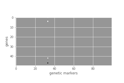
plt.figure();
plt.imshow(B, cmap=plt.cm.Greys_r);
plt.xlabel('genetic markers');
plt.ylabel('genes');

From the above visualization of B, you can see that a single variant influences the expression of four genes. This is known as a hotspot.

In order to process the above data, we proceed as follows:

import eQTLseq as seq

Z_norm = Z / seq.calculate_norm_factors(Z)        # normalize data
Z_trans = seq.transform_data(Z_norm, kind='log')  # transform data

## run Gibbs sampler
rnd.seed(0)
res = seq.run(Z_trans.T, G, n_iters = 4000, burnin=0.5, model='Normal', n_threads=1)

So, after normalizing and log-transforming the data, we pass it to function run, which runs for 4000 iterations (n_iters=4000), rejecting the first half as burn-in (burnin=0.5). Notice that the expression matrix Z_trans is first transposed and then passed to run, because this function requires a samples x genes expression matrix and a samples x genetic markers matrix of genotypes. We use a Normal model (model=Normal) and, since we have a relatively small number of genes, we only use a single thread (n_threads=1). The normalization factors (calculate_norm_factors) are computed using the relative log expression (RLE) method, which is also used by DESeq. Other options for parameter kind in function transform_data are logit, arcsin, blom and boxcox. Transforming the data is necessary, if model=Normal. Other options for model are Poisson, Binomial and NBinomial, in which case data transformation is not necessary.

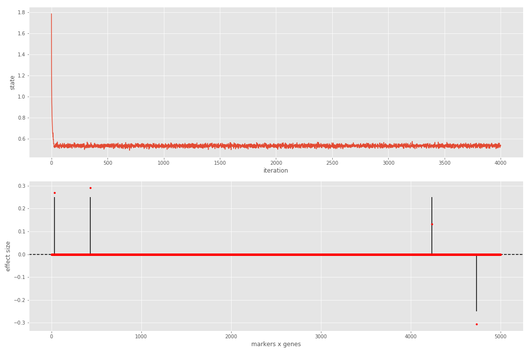
After the sampler finishes, we can visualize the results as shown below:

## normalize beta
Bhat = res['beta']
Bhat = Bhat / nmp.abs(Bhat).sum()
Bnorm = B / nmp.abs(B).sum()

## plot
plt.figure(figsize=(15,10))

plt.subplot(2,1,1);
plt.plot(res['state'][1:]); plt.xlabel('iteration'); plt.ylabel('state')

plt.subplot(2,1,2);
plt.vlines(range(Bnorm.size), 0, Bnorm.ravel());
plt.axhline(linestyle='--', color='k');
plt.plot(Bhat.ravel(), 'r.'); plt.xlabel('markers x genes'); plt.ylabel('effect size');

## compute metrics
metrics = seq.calculate_metrics(Bhat, Bnorm)
print([metrics[_] for _ in ('MCC', 'FDR')])

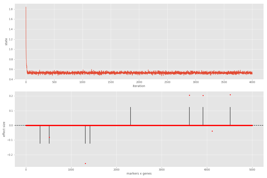
We can see that the sampler reaches steady state very quickly and that all true associations have been detected. If we repeat the process for a more complicated dataset, the results are contaminated with a single false positive.

In practise, we can reject all discoveries below a threshold (e.g. 25% of the maximum in magnitude effect size). We can enforce this condition in the computation of metrics (last two lines of the above code) as follows:

metrics = seq.calculate_metrics(Bhat, Bnorm, beta_thr=0.25)
print([metrics[_] for _ in ('MCC', 'FDR')])

We can see that this takes care of the false positive, thus benefiting the metrics.

dvav/eQTLseq

Hierarchical probabilistic models for multiple gene/variant associations based on NGS data

Installation

Usage