Gregory Way1, Casey Greene1, Yolanda Sanchez2
- University of Pennsylvania
- Geisel School of Medicine at Dartmouth
Patient derived xenograft (PDX) models were derived from primary and metastatic tumors from patients admitted to Dartmouth-Hitchcock Medical Center (DHMC) with pancreatic adenocarcinoma (PAAD). The PDX models and tumor samples were whole exome sequenced (WES) to determine how the mutations from primary tissue and metastases propagate and evolve. The following repository outlines the wes and analysis pipelines.
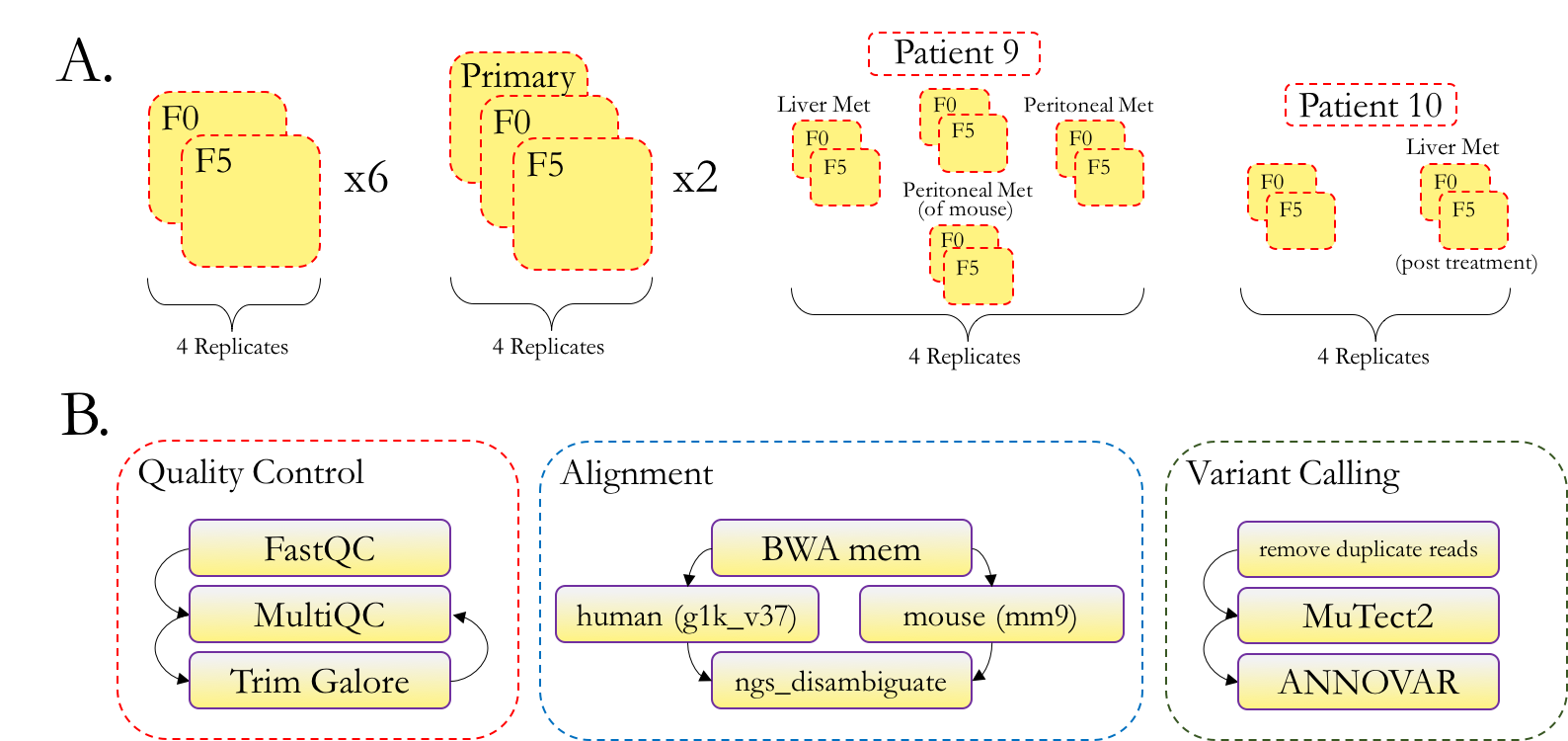
This is a tumor-only analysis; there were no pooled or patient-matched normal samples available. The following flowchart summarizes the wes pipeline.
Figure 1A describes the technical replicates and data-types available across tumor and mouse passages. Figure 1B outlines our whole exome sequencing pipeline. We first apply quality control processing to raw reads, then align and remove mouse reads, and finally call and annotate variants.
See wes_pipeline.sh for our current variant-calling pipeline for tumor-only WES.
This script was run step-by-step on the Dartmouth Discovery compute cluster.
All work was performed using the Dartmouth Discovery Cluster Computer with the conda environment specified in environment.yml.
There are 3 major steps this repository provides to get from raw sequencing reads to annotated variants.
1. Setup reproducible computational environment (setup_environment.sh, install.sh)
# Setup conda (version 4.5 or greater) environment
bash setup_environment.sh

# NOTE: run `conda activate pdx-exomeseq` at the beginning of each session

# Install dependencies and initialize files
# This includes downloading reference genomes and generating several index files
bash install.sh
2. Run data processing pipeline (wes_pipeline.sh)
# NOTE: the commands in the following script must be run sequentially
# The script will submit several jobs per specified file that can take upwards of
# 12 hours per sample to run _for each command_. This requires the user to specify
# which command is being run by commenting out all others.
bash wes_pipeline.sh
Also note that the configuration file discovery_variables.yml includes absolute paths to each tool or resource.
It is sufficient to update this file only if paths to current tools change.
3. Visualize and summarize results (analysis_pipeline.sh)
We use Jupyter notebooks and R scripts to visualize and summarize results. We describe the analysis in the next section.
After obtaining the called variants, we perform a series of analyses and visualizations.
These analyses use a separate conda environment which is specified in
analysis_environment.yml.
Follow these steps to install and begin using this conda environment:
# Using conda version 4.5 or greater
conda env create --force --file analysis_environment.yml
conda activate pdx-exomeseq-analysisIn order to reproduce the results of the analysis pipeline perform the following steps. (Note that the variants are expected to be processed before running the pipeline)
bash analysis_pipeline.shThe following notebooks perform the analysis and obtain figures and results:
| Script | Output |
|---|---|
1.read-depth-stats.ipynb |
Determine read depth against proportion of genome covered |
2.disambiguate-reads.ipynb |
Visualizing the separation of mouse and human reads |
3.filter-variants.ipynb |
Visualize variant filtration and process filtered VCFs |
4.variant-allele-frequency.ipynb |
visualize gnomAD by SIFT scores for replicates and filtered merged files |
5.upset-plots.ipynb |
Generate UpSet plots to visualize variant overlaps across patient sets |
6.generate-oncoprint-data.ipynb |
Wrangle variant calls to generate data for input into oncoprint visualization |
7.visualize-oncoprint.ipynb |
Visualize oncoprint diagrams and variant similarity matrices |
